7 Branching & Looping II – Complex Programs
Previous chapters have introduced the major building blocks of a MATLAB program – array operations, branching, looping, input/output, and user-defined functions. The challenge of programming is combining these blocks in intelligent ways to solve a problem. It is not always easy; like any other skill, becoming proficient requires practice and struggle. This chapter presents some examples that illustrate how to think about constructing a moderately complex program that fulfills its intended purpose, without unnecessary code or excessive computation.
7.1 Idea of an Algorithm
An algorithm is a sequence of steps, defined in advance, for solving a problem. A program is an implementation of an algorithm; the same algorithm may have a number of different implementations. Before writing a program, it is a good practice to define the algorithm precisely, either by diagramming it with a flowchart, or by writing a pseudocode description of it.
There may be numerous algorithms that can be applied to a given problem, and there may be trade-offs in deciding which one is “best”. For example, there are numerous algorithms for sorting a list of items; computer science students typically study all of them in depth to gain an understanding of these concepts. When evaluating how “good” and algorithm is, there are several considerations:
- correctness – does the algorithm produce a correct result? If the answer to this question is “no”, none of the other questions matter – the algorithm must be rejected.
- completeness – does the algorithm work in all possible circumstances, including special cases? A common source of software bugs is not anticipating all of the conditions (e.g. combinations of inputs) that the program must handle. For example, a bad sorting program may give a fatal error when presented with an empty list to sort, or may not work correctly if the list contains duplicate items.
- compactness – can the algorithm be implemented in code that is compact enough to be understood and maintained easily?
- efficiency – do the time and memory required to execute the algorithm scale reasonably with the size of the problem? An inefficient algorithm may be fine for sorting 1,000 items but hopelessly impractical for sorting 1,000,000 items.
An important point related to MATLAB programming in particular is that there are thousands of built-in functions, which are almost always more efficient than anything that a novice programmer could write. In most cases, it makes no sense to write a sorting program from scratch rather than use the built-in function, sort(), except as an educational exercise. Before investing time in developing an algorithm, it is wise to check whether there is a built-in function that can perform the task.
Video 7.1: Idea of an Algorithm
7.2 A First Example – Guessing the Number
In the previous chapter we used the “guess the number” game as an example of a conditional loop with an if structure within it. The objective in that case was to write a program for a human player. Here we look at it from the opposite perspective – an “artificial intelligence” program to play the game. This time, the human will choose the number, and the computer will try to guess it.
As with any problem-solving exercise, certain things are given or must be taken for granted. In this case, the following is given:
- the range of numbers is between 1 and N, where N is a parameter that determines the difficulty of the game
- after each guess by the computer, the human will enter a response indicating whether the guess is too high, too low, or correct
- the computer gets unlimited guesses
Further, we will assume that the human player will not cheat (although a more sophisticated program could perhaps detect cheating by evaluating whether the human’s responses are consistent).
A very high-level description of the program, without any details of the specific algorithm, is as follows:
- computer prompts the user for the value of N
- computer tells the player to choose a number between 1 and N and hit enter when ready
- computer makes and displays its guess, and asks user to indicate whether it is too high, too low, or correct
- user enters response
- if not correct, go back to step 3; otherwise, game over
Step 3 glosses over the most important detail: how does the computer decide on its next guess? We present 3 possibilities, from a very bad algorithm, to a slightly better one, to a good one.
7.2.1 Bad Algorithm – Random Guessing
The simplest, most inefficient algorithm is to guess randomly using the built-in pseudo-random number generator (i.e. the randi() function). If the previous guess was too low, the next guess is chosen randomly between the previous guess and N; otherwise, it is chosen between 1 and the previous guess. A MATLAB implementation of this algorithm is shown below.
% Guess the number - AI version: random guessing
% The user picks an number, and the computer tries to guess it
% Get game parameters from the user
game_level = input('Do you want to pose an easy (1), medium (2), or hard (3) challenge?')
upper_limit = 10^game_level;
fprintf('Pick a number between 1 and %i\n', upper_limit);
fprintf('Hit enter when ready');
pause();
%initial guess is the middle of the range
guess = round(upper_limit/2);
%Keep guessing until you get it right
is_correct = false;
while ~is_correct %this is the same as while is_correct == false
fprintf ('My guess is %i\n', guess);
response = input ('Enter 1 if my guess is too high; -1 if it is too low; 0 if correct:')
switch response
case -1
guess = randi ([guess+1, upper_limit])
case 1
guess = randi ([1, guess-1])
case 0
is_correct = true;
otherwise
%if user enters anything else, quit the game
break;
end
end
What makes this algorithm especially inefficient is that it does not keep track of information from previous guesses. As a result, there is no upper limit on the number of guesses required to find the answer; the average number of required guesses is approximately N/2.[1] A break statement can be used to terminate the loop as shown to keep the game from dragging on endlessly.
Of course the algorithm could be improved by keeping track of the previous guess history, at the expense of increased programming complexity. For purposes of this discussion, we chose to keep it as simple (and inefficient) as possible.
7.2.2 Better Algorithm – Incremental Change
Another simple but inefficient approach is to increase or decrease the guess by 1 each time. This is guaranteed to work – if the number of guesses is unlimited – but will require a large number of guesses on average. If the initial guess is N/2, and the human player’s selection of the number is truly random, the average number of required guesses is N/4 – only a factor of 2 better than random guessing. However, there is now an upper limit on the number of guesses, which is N/2 – a big improvement. A MATLAB implementation is shown in the following example. Note that only two lines have changed from the previous program.
% Guess the number - AI version: incremental guessing
%Initialization portion omitted for brevity - same as previous
%initial guess is the middle of the range
guess = round(upper_limit/2);
%Keep guessing until you get it right
is_correct = false;
while ~is_correct %this is the same as while is_correct == false
fprintf ('My guess is %i\n', guess);
response = input ('Enter 1 if my guess is too high; -1 if it is too low; 0 if correct:')
switch response
case -1
guess = guess + 1;
case 1
guess = guess - 1;
case 0
is_correct = true;
otherwise
%if user enters anything else, quit the game
break;
end
end
7.2.3 Good Algorithm – Bisection Search
The previous two algorithms have different flaws: the first one did not keep track of and use information that was available to it – the results of previous guesses – and the second was too timid in choosing the next guess, so that it only ruled out one number at a time. There is an approach, bisection search, that resolves both of these shortcomings. It uses the prior results to bracket the number that it is searching for between upper and lower limits, and adjusts the guess in such a way that it reduces the bracketed range each time.
The operation of this algorithm is illustrated in the presentation below.
Presentation 7.2: Bisection Search
Checkpoint 7.1: Bisection Search
The bisection search algorithm is much more efficient than random guessing or incremental changes. In fact, the upper limit on the number of guesses is log2(N), which means that it scales less than linearly with N. The larger N is, the greater the advantage offered by this method over the previous ones.
A MATLAB implementation for the bisection search algorithm is shown below.
% Guess the number - AI version: bisection search
%Initialization portion omitted for brevity - same as previous
%initial guess is the middle of the range
guess = round(upper_limit/2);
%Keep guessing until you get it right
is_correct = false;
while ~is_correct %this is the same as while is_correct == false
fprintf ('My guess is %i\n', guess);
response = input ('Enter 1 if my guess is too high; -1 if it is too low; 0 if correct:')
switch response
case -1
lower_limit = guess + 1;
case 1
upper_limit = guess - 1;
case 0
is_correct = true;
otherwise
%if user enters anything else, quit the game
break;
end
%next guess is mid-point of the upper and lower limits
guess = round((upper_limit + lower_limit)/2);
end
Another Application of Bisection Search – Finding a Name in a List
The bisection search technique can be used in a number of applications, including root finding and searching for an item in an ordered list. The presentation below illustrates its application to finding a name in an alphabetized list. Writing the code to implement it is left as an exercise.
Video 7.1: Bisection Search
Checkpoint 7.2: Name Search
A Second Example – Maximizing Bill Payments
The previous chapter introduced the problem of paying a number of bills with a limited bank balance. Our approach at that time was simply to pay the bills in order until the balance was depleted, ensuring that the “highest priority” bills would be paid. We could have chosen a different objective – maximizing the number of bills paid, or the total amount paid. Let’s approach the problem again, this time with the objective of minimizing the total dollar amount of unpaid bills – in other words, maximizing the dollar amount paid.
We will call the previous chapter’s approach of paying the bills in order the “simple” algorithm, since we are not giving any thought to what might produce a better solution. That program is repeated below:
%Bill paying program - simple algorithm
%values must have been assigned to the individual variables (mortgage, car, etc.) previously
bills = [mortgage, car, electricity, water, gas, insurance, cable];
for j = 1:length(bills) %loop over all bills
%if the balance is sufficient to pay the next bill, pay it
%otherwise, just go to the next bill
if balance > bills (j)
balance = balance - bills(j); %deduct that amount from the account balance
end
end
The next approach is a “greedy” algorithm – that is, always pay the largest remaining bill that is less than or equal to the remaining balance. Intuitively, it seems likely that the greedy algorithm will increase the total payments relative to the simple algorithm. It is likely, but not guaranteed. Consider this example:
initial balance = 900
bills = {550, 325, 800}
The simple algorithm pays the first two bills, for a total of 875, while the greedy algorithm pays the 800 bill first and only.
On the other hand, here is an example in which the greedy algorithm does indeed produce a higher total than the simple algorithm:
initial balance = 1150
bills = {550, 325, 800}
The simple algorithm again pays the first two bills, for a total of 875, but the greedy algorithm pays 800 + 325 = 1125.
Greedy Algorithm with Sorting
A trivial way to implement the greedy algorithm is to sort the bills in descending order, then apply the simple algorithm. Since MATLAB has a built-in sort() function, it is only necessary to add one line to the previous program:
bills = sort(bills, 'descend'); %default is ascending order
(If it is desired to preserve the original list of bills, a second array could be used instead of overwriting the variable bills.)
Checkpoint 7.3: Greedy Algorithm
Greedy Algorithm without Sorting
A more challenging problem is to implement the greedy algorithm without sorting. Sorting is a fairly computationally intensive operation, so in some circumstances, especially if the list of items is changing rapidly, it might not be feasible to sort repeatedly.
If the list of items (bills, in our example) is not sorted, then the algorithm must search the entire list to find the largest bill that is less than the remaining balance each time a bill is paid. In other languages, nested loops would probably be necessary, but in MATLAB it can be done more efficiently using a logical array operation and the max() function:
%find the largest bill that is less than or equal to the remaining balance
next_to_pay = max(bills (bills <= balance));
Once the amount of the next bill to be paid is determined, that bill must be removed from the list, so that it is not paid again. One way to determine which bill to remove from the list is with the find() function. There may be multiple bills of the same amount, but we only want the first one:
j = find(bills == next_to_pay, 1, 'first'); %find the index of the next bill to pay
balance = balance - bills(j);
bills (j) = []; %remove that bill from the list after it is paid
An important caveat: in this case, the bills have integer values, so it is OK to use the == operator in the find statement. If they were floating-point values, it would be safer to use abs(bills-next_to_pay)<0.01 to avoid problems with roundoff error.
Checkpoint 7.4: Greedy Algorithm without Sorting
Optimal Solution – Brute-Force Algorithm
Neither the simple nor the greedy algorithm is guaranteed to find the optimal solution that maximizes the bill payments. For the previous checkpoint question, with
initial balance = 1690
bills = {375, 175, 225, 45, 325, 1150}
The optimal solution is 1150 + 325 + 225 = 1650.
Is there an algorithm that is guaranteed to find this optimal solution? There is, but it is inefficient and so is only practical if the number of bills is around 10 or less.
This “brute-force” approach is based on the fact that the result of the simple algorithm depends on the order in which the bills are listed. In the previous example, if the bills happened to be listed in this order:
bills = {1150, 325, 225, 375, 175, 45}
the simple algorithm would find the optimal solution, which is to pay the first 3 bills.
Since there are some permutations of the bills that would enable the simple algorithm to find the optimal solution, the brute-force algorithm simply applies the simple algorithm to all permutations, and keeps the best result. Unfortunately the number of permutations of N items is N!, which scales badly with increasing N. There are 120 permutations of 5 items, over 3.6 million permutations of 10 items, and more than a trillion permutations of 15 items. Consequently, this algorithm isn’t really practical, since it becomes intractable for a rather modest number of items.
There is a MATLAB built-in function, perms(), to generate all permutations of an array. The function generates a matrix, with one permutation stored in each row; for example, if perms() is applied to the list of bills given previously, the first few rows of the matrix are as shown:
>>perms(bills)ans =1150 325 45 225 175 3751150 325 45 225 375 1751150 325 45 175 225 3751150 325 45 175 375 2251150 325 45 375 225 1751150 325 45 375 175 2251150 325 225 45 175 3751150 325 225 45 375 1751150 325 225 175 45 3751150 325 225 175 375 451150 325 225 375 45 1751150 325 225 375 175 451150 325 175 45 225 3751150 325 175 45 375 2251150 325 175 225 45 3751150 325 175 225 375 451150 325 175 375 45 2251150 325 175 375 225 451150 325 375 45 225 1751150 325 375 45 175 225function bills_paid = simple_pay (bills, balance)%Bill paying function - simple algorithm
bills_paid = 0; %initialize total paid
for j = 1:length(bills) %loop over all bills
%if the balance is sufficient to pay the next bill, pay it
%otherwise, just go to the next bill
if balance > bills (j)
balance = balance - bills(j); %deduct that amount from the account balance
bills_paid = bills_paid + bills(j); %keep track of total paid
end
end
end
A program to apply the simple_pay() function to each permutation and find the optimal solution is the subject of the next check-point question.
Checkpoint 7.5: Brute-force Algorithm
You may be left wondering, is there an algorithm that is guaranteed to find the optimal solution but is more practical for larger values of N? There is, but the code is substantially more complicated [2], so we choose not to discuss it here. As an exercise, you might try posing the question to a generative AI tool like Copilot or ChatGPT.
Looping over 2D Arrays
As we pointed out at the very beginning, the “MAT” in MATLAB stands for “matrix.” MATLAB was created to perform matrix operations efficiently, and it has numerous features and built-in functions to do. Consequently, it is not often necessary to loop over all of the elements of a matrix. Nonetheless, it is an important skill, both because writing loops is often easier for novice programmers than using array operations skillfully, and because in other programming languages – and occasionally even in MATLAB – it may be the only option.
A common approach to iterating over matrix, element-by-element, is to use nested for loops – the outer loop iterates over the rows, and the inner loop iterates within a given row (or vice versa). As a trivial example, consider creation of a MxM multiplication table. The objective is to create a matrix in which the rth row, cth column element is r*c. This can be created using nested for loops as follows:
% Assume that the variable M has already been defined
for r = 1:M %loop over all rows
for c = 1:M %loop over all columns
mult_table(r,c) = r*c;
end
end
The most important thing to understand about nested loops is that the inner loop goes through its entire sequence each time the outer loop executes. The total number of executions in this example is therefore M2.
Whenever an array is created element-by-element this way, it is advisable to initialize the array to all zeros if possible. This improves the execution speed of the program, since allocation of the memory to store the matrix can be done once at the beginning, rather than repeated on each iteration of the loop. This can be done using the zeros() function:
%Allocate memory for the matrix prior to the loop
mult_table = zeros(M,M);
A further improvement in efficiency can be gained by taking advantage of the symmetry of the matrix; since j*k = k*j, the number of executions of the loop can be reduced by adding the (c,r) element of the matrix at the same time as the (r,c) element:
%within the inner loop:
mult_table(r,c) = r*c;
mult_table(c,r) = mult_table(r,c);
With this change, the inner for statement can be changed to
for c = r:M %cols 1:r-1 have already been assigned
The following example puts all of this together and shows how the program executes, step-by-step, using M = 3:
As a less trivial example, consider creation of a matrix containing Pascal’s triangle. Although it is not the traditional representation of the triangle, we will use a lower-triangular matrix. A limitation of this approach is that the “empty” elements of the triangle will contain zeros.[3]
%Initialize matrix to zeros for efficiency
pascal_triangle = zeros(N,N);
for row = 1:N
%first and last element of each row are 1s
pascal_triangle (row, 1) = 1;
pascal_triangle (row, row) = 1;
%other elements are the sum of the two elements above them
for col = 2:row-1
pascal_triangle (row, col) = pascal_triangle(row-1, col-1) + pascal_triangle(row-1, col)
end
end
As with the multiplication table, the number of iterations can be reduced by taking advantage of the symmetry of the matrix, as shown below. Understanding how indexing is used in this example may require some thought.
Cellular Automata and Conway’s Game of Life
Mathematicians and computer scientists have long studied the problem of how complex, global behavior can arise from simple, local rules. For example, each neuron in a brain makes a local decision to fire or not based only on its local environment, but the collective actions of these cells leads to complex behavior by the organism.
One approach to modeling this type of phenomenon is called “cellular automata”. In the most basic type of CA algorithm, the “universe” or “organism” is represented by a grid of logical values (1 or 0). Each cell of the grid repeatedly transitions from its current state to its next state based on a simple set of rules involving only itself and its nearest neighbors.
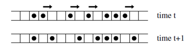
An example of a CA algorithm can be seen in a simple model of traffic flow. The road acts like the “organism” and is split into finite cells. Each cell is either occupied by a vehicle (a logical 1) or unoccupied (a 0). In each time step, a car advances if and only if the cell ahead of it is unoccupied. The rules for updating cells are as follow (the kth cell at time t):
- If cell(k, t) = 1 and cell(k+1, t) = 1, then cell(k, t+1) = 1 (the car stays where it is)
- If cell(k, t) = 1 and cell(k+1, 0) = 0, then cell(k, t+1) = 0 (the car moves to the next cell)
- If cell(k, t) = 1 and cell(k+1, t) = 0 and cell(k-1, t) = 1, then cell(k, t+1) = 1 (The car moves to the next cell, and the car in the previous cell moves into the cell)
- If cell(k, t) = 0 and cell(k-1, t) = 1, then cell(k, t+1) = 1 (the car from the previous cell moves into this one)
- If cell(k, t) = 0 and cell(k-1, t) = 0, then cell(k, t+1) = 0
- Etc.
This set of conditions sounds very complicated, but it can be summarized by the following logical expression:
cell(k, t+1) = cell(k, t) & cell(k+1, t) | ~cell(k, t) & cell(k-1, t)
Typically, all cells are updated simultaneously. This process is illustrated in the figure below.[4]
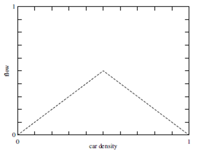
As simplified as this model is, it can capture some important general features of traffic flow. For example, the flow rate (number of cars passing a given point per unit time) as a function of traffic density can be computed. The result will be as shown in the graph below.[5] In light traffic, adding more cars to the road increases the traffic flow, but once a critical density is reached, adding more cars decreases the traffic flow (due to congestion).
One of the most famous applications of cellular automata is Conway’s Game of Life. In this model, the universe is a 2-dimensional grid in which each cell is regarded as “alive” (1) or “dead” (0). The cells are updated based on how many of its 8 nearest neighbors are alive according to the following rules:
- if there are less than 2 live neighbors, the cell dies (becomes 0).
- if there are exactly 2 live neighbors, the state of the cell does not change.
- if there are exactly 3 live neighbors, the becomes or remains alive (1)
- if there are more than 3 live neighbors, the cell dies (becomes 0)
These rules are summarized in the table below.
| Number of Live Neighbors | Current State of Cell | Next State of Cell |
| 0-1 | 0, 1 | 0 |
| 2 | 0 | 0 |
| 2 | 1 | 1 |
| 3 | 0, 1 | 1 |
| 4-8 | 0, 1 | 0 |
Despite having exceedingly simple rules, this algorithm can give rise to quite complex behavior, which is precisely the point – to demonstrate how complex, global phenomena can be modeled by simple, local interactions. In fact, it has been shown formally that anything that can be computed by a classical computer can be computed by this algorithm!
A MATLAB function to implement this algorithm is given below. The function takes a matrix of 0s and 1s as input, and returns the modified matrix. Note:
function [ out_grid ] = LifeSimulation( in_grid )
% Function to apply Conway's Game of Life Algorithm
% Input = matrix of 0s and 1s representing the "universe"
% Output = modified matrix describing the universe in the next frame
% Uses fixed boundary conditions - edges of the matrix are not modified
N = size(in_grid); %Determine the size of the matrix
%*******************************************
% Important: make a copy of the matrix
% Calculate number of neighbors from the OLD matrix
% Make modifications in the NEW matrix
%*******************************************
out_grid = in_grid;
% loop over rows & columns, skipping the edges
for row = 2:N(1)-1
for col = 2:N(2)-1
% count the number of live neighbors: sum the 3x3 sub-matrix
% centered on the current cell and subtract the current cell itself
% sum(sum(...)) sums the ENTIRE matrix; could also use sum(..., 'all')
live_neigh = sum(sum(in_grid(row-1:row+1, col-1:col+1)))-in_grid(row,col);
%Apply the rules based on the number of live neighbors
switch live_neigh
case {0, 1} % less than 2 live neighbors - cell dies of loneliness
out_grid(row,col) = 0;
case 2 % 2 live neighbors - no change
out_grid(row,col) = out_grid(row,col); %don't need this; just for completeness
case 3 % 3 cell is resurrected
out_grid(row,col) = 1;
otherwise %more than 3 - cell dies of overcrowding
out_grid(row,col) = 0;
end
end
end
end
The result of applying this matrix to a simple test pattern is shown below. This pattern is called a “blinker” because as the Life algorithm is applied repeatedly, it oscillates between a vertical and horizontal pattern.
>> blinkerMatrix = [zeros(1,5); 0 0 1 0 0 ; 0 0 1 0 0; 0 0 1 0 0; zeros(1,5)]blinkerMatrix = 0 0 0 0 0 0 0 1 0 0 0 0 1 0 0 0 0 1 0 0 0 0 0 0 0>> LifeSimulation(blinkerMatrix)ans = 0 0 0 0 0 0 0 0 0 0 0 1 1 1 0 0 0 0 0 0 0 0 0 0 0>> LifeSimulation(ans)ans = 0 0 0 0 0 0 0 1 0 0 0 0 1 0 0 0 0 1 0 0 0 0 0 0 0
The next checkpoint question steps through a portion of the algorithm.
Checkpoint 7.6: Game of Life
Problems
- Image Quantization
| Original Pixel Value | New Pixel Value |
| 0 – 64 | 0 |
| 65 – 128 | 1 |
| 129 – 192 | 2 |
| 193 – 255 | 3 |
-
-
- If that letter matches the letter in the same position of the target word, +1
- If that letter is in the target word, but not in the same position, 0 (Hint: a relational operator with the sum function is the easiest way to do this.)
- If that letter is not in the target word, -1
-
-
- plant_names, a string array with the names of the varieties
- plant_nums, a numerical array with the number of available plants (that is, how many successful seed starts there are for each variety)
- max_plants, a randomized integer with the number of spaces available in the garden.
-
- Starting at index 1, loop through the numerical array
- If there are any remaining spaces in the garden and any remaining plants of that type
- add the name of that variety to plant_choices
- subtract 1 from max_plants
- subtract 1 from the correct element of plant_nums
- go to the next plant in the list (i.e. increase the index by 1)
- When you get to the end of the array, if there are still remaining spaces, go back to step 1
- Exit the loop when there are no remaining spaces.
Place these lines at the beginning of your program to generate the plant information:
plant_names = ["Brandywine", "Roma", "Beefsteak", "Cherokee Purple", "Giant Syrian", "Oxheart","Garden Leader Monster",..."Serrano", "7-Pot Chocolate", "Thai Chili", "Sugar Rush Red", "Orange Bell", "Mitoyo", "Senshu Kinukawa Mizu", "Kurume Long"];plant_nums = randi([2,6], size(plant_names));max_plants = randi([20,30]);fprintf('You have %i plants, but only %i spaces\n', sum(plant_nums), max_plants)a) Copy the earlier function to the bottom of your script as a local function.
b) Download this file and read it into MATLAB using a the load command word_matrix.mat It provides an 11×33 matrix representing a 3-letter word. Apply your function to the provided matrix, 11 columns at a time, to identify the 3 letters.
c) Store the resulting word in a character array and print it to the command window with a suitable message.
-
- Given an MxM image matrix, where M is divisible by N
- Starting at the upper left corner (1,1), loop over the columns and rows, using nested for loops, in steps of N
- Extract the NxN submatrix with the current row & column as the upper left corner
- If the majority of the pixels in that submatrix are 1s, then the corresponding pixel of the output matrix is 1; otherwise it is 0
puppyBW in the workspace, but it will not be square. To fit the specifications of the problem, create a square matrix as follows:puppyBW_square = puppyBW(:, 1:300);puppyBW_square as the input to your function.imshow() to show the two images in a single figure using subplot. They should resemble these:
-
- Given an NxM input matrix
- Make a copy of the matrix – this will be the output matrix
- loop over rows 2 to N-1 of the input matrix
- loop over columns 2 to M-1 of the input matrix
- take the average of the 3×3 submatrix centered on the current row & column
- set the corresponding element of the output matrix equal to this average
You can use this code to generate a simple test image, consisting of a cross pattern.
Image1 = zeros(10,10);Image1(2:9, 5:6) = 1;Image1(5:6, 2:9) = 1;imshow() to display the original and smoothed images. If your function is correct, they should resemble these:
Find an error? Have a suggestion for improvement? Please submit this survey.
- This is not easy to prove rigorously, but it is simple to verify by writing a program to run a large number of trials. ↵
- A note about terminology: when computer scientists talk about the complexity of an algorithm, they don't mean how complicated the code is. They mean how do the memory and CPU time requirements scale with the size of the problem. So the brute force algorithm discussed above has a complexity of N! There are other algorithms that have a complexity of N2 ↵
- There is another data structure called a cell array that allows elements to be truly empty. Cell arrays are covered in Chapter 11. ↵
- Adapted from the online course, “Simulation and Modeling of Natural Phenomena” from University of Geneva ↵
- ibid ↵
