14 Numerical Computing

Since this book (and the course it was originally based on) focuses on programming, it has not emphasized MATLAB’s many built-in capabilities for performing mathematics. In reality, it is almost always smarter to use “canned” routines for performing complex computations, since many hours of development have gone into ensuring their accuracy and efficiency. While writing a simulation from scratch using Euler’s method is a valuable educational exercise, it is not the best use of a practicing engineer’s time, when MATLAB has functions to perform the calculation with minimal programming.

This chapter covers some of MATLAB’s built-in functions for several kinds of fundamental engineering analysis:

• curve fitting
• interpolation
• solving a system of linear equations
• solving an ordinary differential equation
• optimization and parameter estimation

14.1 Polynomial Curve Fitting

Extracting information from experimental data is a fundamental task in engineering analysis. A basic technique for accomplishing that is to fit a curve describing a theoretical relationship to the data. The standard approach is least-squares fitting, in which the model parameters (e.g. the coefficients of a polynomial) are chosen to minimize the sum of the squares of the differences between the theoretical curve and the experimental points. MATLAB has a built-in function, polyfit(), to perform least-squares fitting with polynomial models. The input arguments are the x and y data arrays and the order, n, of the polynomial. The output argument is an array containing the coefficients of the polyomial.

As a first example, consider a linear fit to a set of deflection vs. load data for a cantilever beam and extraction from the elastic modulus from the slope of the line. The theoretical relationship between deflection, [latex]\Delta y[/latex], and the applied load, P, for an end-loaded cantilever beam having an elastic modulus E is:

[latex]\Delta y = \frac{PL^3}{3EI}[/latex]

where L is the free length of the beam, and I is the area modulus of elasticity, which depends on the cross-sectional area and shape of the beam. For a solid rectangular beam of width w and height h

[latex]I = \frac{1}{12}wh^3[/latex]

A common first-year engineering experiment is to measure the deflection of a beam for several applied loads. A plot of [latex]\Delta y[/latex] vs. P should be a straight line with slope

[latex]m = \frac{L^3}{3EI}[/latex]

Suppose the experimental data are as given in arrays delta_y and P. The coefficients of the least-squares line are calculated by the polyfit() function as follows:

coeffs = polyfit(P, delta_y, 1);

The third argument, 1, indicates that it is a first-order (linear) polynomial. The function returns a vector of coefficients in descending order; in this case coeffs(1) is the slope, and coeffs(2) is the y-intercept.

Once the coefficients of the fitted linear are determined, a plot of that line can be created with the help of the polyval() function. This function takes as inputs the vector containing the coefficients and an array of x-values at which the corresponding y-values are to be calculated. It returns the vector of y-values, which can be used to plot the curve. The example below shows the complete process of fitting a straight line, generating a plot of the data overlaid with the best-fit line, and calculating the elastic modulus based on the slope.

14.1.1 Choosing a model

Curve fitting requires choosing an equation to describe the data, which means asserting some theoretical relationship (model) between the dependent and independent variables. The choice of model should be driven by an understanding of the physics (or chemistry or other foundational discipline) of the problem. A choice of model should not be driven entirely by the desire to get a “good fit” to the data.

To illustrate this point, consider some data for the position vs. time of a free-falling object, released from rest. We know from elementary physics that, excluding air resistance, this should be a quadratic relationship. But with imperfect data, there may be a temptation to use a higher-order polynomial, just to achieve a closer fit to the data. Consider this example, in which random variation has been added to some simulated data:

Figure 14.1: Curve Fitting with Noisy Data

The cubic curve gives a better fit to the data, in the sense that it has a higher R² value, but that does not mean that it is the right model to use. What would be the physical meaning of the cubic term? Unless it is reasonable to propose that the acceleration of gravity varies significantly over a distance of 500 meters from the surface of Earth (it does not), the extra term is just an artifact of the noise in the data. As one of my professors told me when I made the error of adding an extra parameter into a model just to get a better curve fit, “If the parameter doesn’t mean anything, neither does the model.”

14.1.2 Over and Under-fitting

Without an understanding of the problem, it is possible to make the opposite mistake, such as assuming that everything can be fit by a straight line. Here is the same data from the previous example with a linear curve fit:

Figure 14.2: Underfitting of Noisy Data

The R² value is actually not terrible – without knowing that the physics dictates a quadratic model, you might think that this linear model is adequate. Why did we use the more complicated (quadratic) model? Because we can give a reasonable physical explanation for the quadratic term. The linear model in this case is an example of “underfitting” (not using enough parameters for a complete description of the data), while the cubic model is “overfitting” (using extra parameters that have no meaning).

The most important point to take away is that in science and engineering you do not do curve fitting for its own sake, but in order to extract physical parameters from data. ^[1]In the case of the free-falling object, the purpose of the experiment might be to determine the value of the acceleration of gravity. Our physics model says that the quadratic term should be g/2. Looking at the equation of the least-squares curve:

Figure 14.3: Extracting parameters using the equation of the best-fit curve

our experiment gives us a value of 10.4 m/s² for g, which is about 5.8% error compared to the accepted value of 9.81 m/s². The equation also tells us that the initial velocity is 1.9 m/s, which we know is wrong, because we released the object from rest. In fact, this is another extraneous parameter that, while it may improve the R² value, can actually hurt the accuracy of our determination of g.

We can get a better result by changing the way we present the data so that the initial velocity term goes away. To see this, look at this plot in which t² is used as the independent variable – there should now be a linear relationship between the dependent and independent variables, with the linear coefficient being -g/2. This method gives us a value of g = 10.1 m/s², for an error of 2.4 %. Eliminating the extraneous initial velocity parameter gives us a more accurate value for the parameter that we are trying to determine.

Figure 14.4 Transforming the model to eliminate an extraneous parameter (the linear term in the quadratic model)

14.1.3 Non-Polynomial Curve Fitting by Transformation

While many problems can be described by a polynomial equation, sometimes the science dictates a more complicated relation, such as an exponential, logarithmic, or power law. In many cases, it is possible to manipulate the equation so that polynomial curve fitting can be used.

As an example, consider an experiment to determine the half-life of a radioactive isotope. The foundational equation, which was discussed in one of the simulation examples of the last chapter, is:

[latex]\\[/latex]

[latex]N(t) = N_0 \ ^{-\frac{t}{\tau}}[/latex]

[latex]\\[/latex]

To put this equation into a form that can be handled by polyfit, take the natural log of both sides:

[latex]\\[/latex]

[latex]log N = log N_0 - \frac{t}{tau}[/latex]

[latex]\\[/latex]

A plot of log N vs. t will therefore be a straight line with slope = [latex]-1/\tau[/latex] and intercept = log N₀. The time constant can be extracted from a linear fit and the half-life calculated by multiplying by [latex]\log 2[/latex].

14.2 Interpolation

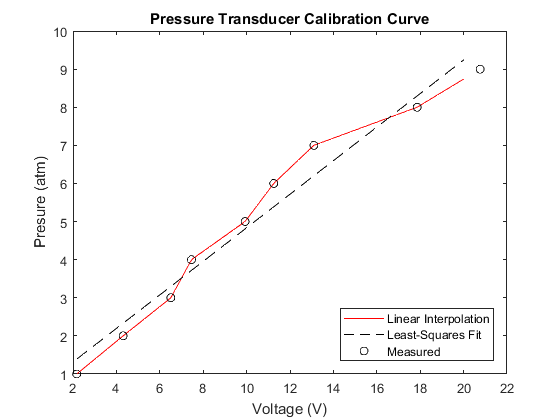
A closely related topic to curve fitting is interpolation, which means estimating the value of a quantity between known values. For example, a transducer – let’s say a pressure sensor – may have been calibrated by making measurements at several known pressure values. Suppose that the calibration data is as follows:

After calibration, an unknown pressure is measured, and the resulting voltage is 56.5 mV. What is the pressure? It must be between 1.0 and 1.1 atm, since the measured voltage is between the voltage measurements at those two calibration points, but what precisely? That depends on the specific interpolation method used; the simplest method is linear interpolation, in which the dependent variable is assumed to vary linearly with the independent variable between data points. See the linked article for details of the calculation.

MATLAB has a built-in function, interp1(), to perform one-dimensional interpolation. It accepts as arguments:

• a vector containing the known x-values
• a vector containing the known y-values
• a vector containing the x-values at which the y-values are to be estimated

For the example of the pressure sensor described above, the function call could be:

>> P = interp1([52.0, 68.3, 79.5], [1.0, 1.1, 1.2], 56.5)

P =

1.0276

>>

The interp1() function can perform other interpolation methods (see the documentation for details). One commonly used method is cubic spline interpolation, which draws a smooth curve through the data points, rather than connecting them by straight lines. To choose spline interpolation instead of linear, an additional argument is passed to interp1() as follows:

>> P = interp1([52.0, 68.3, 79.5], [1.0, 1.1, 1.2], 56.5, 'spline')

P =

1.0222

>>

The example below performs both linear and spline interpolation on a set of data and plots them to illustrate the difference.

14.2.1 Interpolation vs. Curve Fitting

The difference between curve fitting and interpolation is that in interpolation, no assumption is made about the mathematical form of the relationship. The objective is merely to “connect the dots” between data points, either with straight lines or with a smooth curve like a spline (next subsection) that passes through the points.  In curve fitting, a model is chosen for how the dependent and independent variables are related – a straight line, a quadratic, an exponential, etc. – and fit a curve of that type that passes near the data points. Figure 14.1 compares a straight-line curve fit vs. a linear interpolation through some data points.

Figure 14.5: Curve fitting vs. interpolation

14.3 Systems of Linear Equations

One of the most common tasks in engineering is solving a system of linear algebraic equations of the form

[latex]a_{11} x_1 + a_{12} x_2 + a_{13} x_3 + ... a_{1n} x_n = b_1[/latex]

[latex]a_{21} x_1 + a_{22} x_2 + a_{23} x_3 + ... a_{2n} x_n = b_2[/latex]

…

[latex]a_{n1} x_1 + a_{n2} x_2 + a_{n3} x_3 + ... a_{nn} x_n = b_n[/latex]

where a_ij and b_i are known constants, and x_j are the variables to be solved for. We assume that there are exactly as many equations as unknowns and that the equations are linearly independent, so that there is a unique solution.

Solving a system like this in MATLAB involves 3 steps:

1. Put the a_ij coefficients into a matrix as

[latex]A = \begin{bmatrix} a_{11} & a_{12} & a_{13} & ...& a_{1n} \cr a_{21} & a_{22} & a_{23} & ...& a_{2n} \cr ... \cr a_{n1} & a_{n2} & a_{n3} & ...& a_{nn} \end{bmatrix}[/latex]

   2. Put the b_j coefficients into a column vector:

[latex]B = \begin{bmatrix} b_1 \cr b_2 \cr . \cr . \cr . \cr b_n \end{bmatrix}[/latex]

   3. use the MATLAB “left division operator” to generate the solution. This is a single line of code:

x = A \ B

x will be a vector containing the values of the unknowns.

For example, to solve the set of equations:

[latex]x_1 + 2 x_2 + 3 x_3  = 3[/latex]

[latex]4 x_1 – 5 x_2 + 6 x_3  =2[/latex]

[latex]7 x_1 + 8 x_2 + 9 x_3 = 1[/latex]

Requires 3 lines of code:

14.4 Ordinary Differential Equations

Nearly all of the theory that underlies engineering disciplines is expressed in terms of differential equations, that is, equations involving derivatives of physical quantities. Fundamentally, that is a statement about how nature works – nothing changes instantaneously; rather, the rate of change changes instantaneously. For example, when you turn up the control on an electric heater, you don’t immediately change the temperature in the room, you change the rate at which the temperature increases.

In the previous chapter, we discussed computing the solution to time-dependent differential equations through the simplest possible method, the forward Euler method. In most practical applications, there is no need to write such simulations from scratch – MATLAB has built-in solvers to do the computations. The purpose of this section is to demonstrate the use of those solvers.

As a first example, let’s revisit the basic radioactive decay problem. We want to solve this equation for N(t):

[latex]\frac{dN}{dt} = -\lambda N(t)[/latex]

subject to an initial condition

[latex]N(0) = N_0[/latex]

The MATLAB function ode45() is designed to solve first-order differential equations like this. It takes 3 input arguments:

• a handle to a function defining the time derivative
• the time interval over which to compute the solution
• the initial condition

and returns two arrays: time and the quantity solved for (in this case N(t)).

Here is a short script to solve the exponential decay problem:

%set up parameters - decay constant and initial condition

lambda = 0.01;

N0 = 1000;

%Use an anonymous function to define the derivative

dN_dt = @(t, N) -lambda*N

%Call the solver to integrate over a period of 300 seconds

[t, N] = ode45 (dN_dt, [0, 300], N0);

%plot the results

plot(t, N)

title("Radioactive Decay")

xlabel("Time (sec)")

ylabel("Remaining Nuclei")

The resulting plot is:

Notice that there is no need to define the time step – the solver will determine that based on the characteristics of the equation.

This process can be generalized to higher-order problems by setting up the system of equations in matrix form. Consider a multi-step radioactive decay process in which the first species decays into a second one, which in turn decays into a third. The process is described by a pair of equations

[latex]\frac{dN_1}{dt} = -\lambda_1 N_1(t)[/latex]

[latex]\frac{dN_2}{dt} = \lambda_1 N_1(t) - \lambda_2 N_2(t)[/latex]

This can be expressed in matrix form by defining a vector

[latex]X = \begin{bmatrix} N_1 \cr N_2 \end{bmatrix}[/latex]

and a coefficient matrix

[latex]\Lambda = \begin {bmatrix} -\lambda_1 & 0 \cr \lambda_1 & -\lambda_2 \end{bmatrix}[/latex]

The system of equations can then be expressed in matrix form as

[latex]\frac{dX}{dt} = \Lambda X[/latex]

which looks just like the equation of the previous problem, except that X is now a vector, and [latex]\Lambda[/latex] is a matrix.

A MATLAB script to solve this system is as follows:

The resulting plot is

Notice that, since there are now two variables, the initial condition must be provided as a vector of two values. The output, X, will be a matrix in which each column is the solution for one of the two variables – in this case X(:, 1) is N1, and X(:, 2) is N2.

14.5 Optimization

This final section gives a minimal introduction to the subject of optimization. The examples discussed in the video will be of the simplest type, unconstrained optimization, in which the value(s) of one or more parameters are chosen to minimize a function, with no limits placed on the values of those parameters. The MATLAB function fminsearch() performs this operation using a “simplex” method. (See the link at the end of the section for more information.)

One important point to remember when using fminsearch is that it will find a local minimum, not necessarily the global one. The user must provide an initial guess, and the solution to which the optimizer converges may depend on that guess.

14.6 Mathworks Resources

Systems of Linear Equations

Optimization

14.7 Problems

1. 1. In particle motion with constant acceleration, the position vs. time is given by the following equation:

      [latex]$y(t)=y_0 + v_0t + \frac{1}{2}at^2$[/latex]

      Given the position and time data below, fit a quadratic curve and extract the acceleration and initial velocity.

      [latex]\\[/latex]

      t = 0: 0.1: 2.0;

      y = [5.04 5.16 5.28 5.36 5.20 5.02 4.74 4.31 3.87 3.29 2.60 1.78 0.98 -0.06 -1.10 -2.27 -3.59 -4.91 -6.35 -7.90 -9.62];

      [latex]\\[/latex]

      (a) Use the polyfit function to determine the coefficients of the best-fit quadratic curve.

      (b) Calculate the acceleration and initial velocity based on the coefficients.  The acceleration should be close to the accepted value for g in S.I. units.
   2. Given the sparse set of data below, use linear interpolation to generate estimates of y for x = 0: 0.1: 10.0, and plot the interpolated values (solid line) along with experimental points (markers) on the same graph.
      [latex]\\[/latex]

      xmeas = [0,1.3, 2.2, 3.4, 4.0, 5.1, 6.2, 7, 8.1, 9, 10];

      ymeas = [0 0.3193 0.5227 0.7513 0.8415 0.9566 0.9998 0.9840 0.8986 0.7781 0.5985]
      [latex]\\[/latex]
   3. Applying Kirchoff’s rules to the resistive circuit shown in the video results in the set of equations given below. Solve for the currents.

      [latex]\\[/latex]

      [latex]R_1I_1 + R_2I_2 = 15[/latex]

      [latex]R_1I_1 + R_3I_3-R_4I_4 = 0[/latex]

      [latex]R_2I_2-R_3I_3 = 0[/latex]

      [latex]I_1 - I_2 - I_3 = 0[/latex]

      [latex]\\[/latex]

      (a) Set up the coefficient matrix. (Don’t forget to include 0s for missing terms).

      (b) Set up the column vector for the right-hand side.

      (c) Use the left division operator to solve for the currents – compare the results to the circuit simulation result shown in the video.

4. Use ode45 to simulate a a block of mass m sliding down a straight inclined plane with angle θ, tethered to the top by a Hooke’s law spring.

The acceleration is:

[latex]a = g (sin \theta - \mu_k cos \theta) - k \frac{x}{m}[/latex]

where k is the spring constant and [latex]\mu_k[/latex] is the coefficient of kinetic friction. This equation is only valid while the block is moving down the plane; if it reverses direction (which may happen depending on the parameters) the sign of the friction term changes.

Use the following parameters, and run the simulation for 1.0 second. (For the given parameters, this is the time at which the velocity becomes 0.)

[latex]\\[/latex]

m = 1;%kg

k = 9.8696;%N/m

g = 9.81;%m/s^2

theta = 20;%degrees

mu_k = 0.2;

L = 0.75;%m

v0 = 0;%m/s

[latex]\\[/latex]

The state variables are x and v; the equations are

[latex]\dot{x} = v[/latex]

[latex]\dot{v} = a[/latex]

where a is given by the expression for the acceleration above.

Plot x, v, and a versus t on a 3×1 subplot. (ode45 does not return a, but you can calculate a from x.)

5. Parameter estimation can be seen as a minimization problem – the objective is to choose the value(s) of one or more parameters to minimize the difference between estimated and observed results.

In the previous problem, we provided the values of all of the parameters, such as the spring constant and the coefficient of friction. Suppose that you wanted to determine these parameters experimentally, but you had to infer them from measurements of the motion of the block.

You are given this information:

• • The mass of the block and the angle
  • The values of x and v at t = 1.0 second

You want to determine the values of [latex]\mu_k[/latex] and k for which the simulation predicts the correct values for x and v.

You need to create an objective function to minimize, defined by:

[latex]\\[/latex]

[latex]f = (v_{meas} - v_{target})^2 + (x_{meas} - x_{target})^2[/latex]

[latex]\\[/latex]

The easiest way to do this is to structure the simulation function so that it takes  v_target and  x_target as inputs, along with [latex]\mu_k[/latex] and k, and returns the value of f as given above. Then create an anonymous function of [latex]\mu_k[/latex] and k only, and pass this anonymous function to fminsearch.

The definition of the simulation function might be something like this:

[latex]\\[/latex]

 function f = simulate_block(mu_k, k, v_t, x_t)

[latex]\\[/latex]

Copy your code from the previous problem into this function and modify it so that it takes mu_k and k as inputs and returns the error function, f.

The trickiest part is defining the anonymous function, since in this case there are two parameters that are being varied ([latex]\mu_k[/latex]  and k). These must be passed to fminsearch as an array. So the anonymous function definition would be something like:

[latex]\\[/latex]

fmin = @(params) simulate_block(params(1), params(2), v_meas, x_meas);

[latex]\\[/latex]

where params is a vector that contains the values of mu_k and k.

The starting guesses for mu_k and k must also be passed to fminsearch as an array. Use [0.1, 10.0]. (Correct answers: mu_k = 0.2, k = 9.87.)

Find an error? Have a suggestion for improvement? Please submit this survey.