2 Arrays & Data Operations
MATLAB was created to perform matrix algebra, which involves operations on collections of numbers. Thus the concept of an array, a variable containing multiple values, is fundamental in MATLAB.
A MATLAB array can be one-dimensional, in which case it is called a vector, two-dimensional, in which case it is called a matrix, or higher-dimensional. This book will not deal with array dimensions higher than 2. Initially, we will consider arrays of numbers; later we will introduce arrays of characters and strings.
The dimensions of an array are expressed as number of rows X number of columns. For example if an array has 3 rows and 4 columns, its dimensions are 3×4. Fundamentally, a vector is a special case of a matrix, in which one of the dimensions is 1, and a scalar is a 1×1 matrix.
2.1 Creating Vectors
The most explicit way to create a vector is to list the numbers in square brackets, separated by commas, spaces or semi-colons. This simple script creates and stores 3 vectors:
cargo_weights = [253, 129, 88, 42, 111, 27]
vehicle_occupants = [2 1 4 2 3 2 1 1 5]
Stargell_homeruns = [3; 0; 11; 32; 28; 13; 20; 22; 25; 44; 33; 48; 31; 29; 24; 20; 33; 27; 21; 11; 0]
If this script is run, the command line output is as follows:
cargo_weights =
253 129 88 42 111 27
vehicle_occupants =
2 1 4 2 3 2 1 1 5
Stargell_homeruns =
3
0
11
32
28
13
20
22
25
44
33
48
31
29
24
20
33
27
21
11
0
>>
Notice that the first two arrays are displayed horizontally, while the third is displayed vertically. The reason is that in the first two cases, the numbers were separated by commas or spaces – this creates a row vector. In the third case, the numbers were separated by semi-colons; this creates a column vector. A row vector containing N elements has dimensions 1xN, while a column vector has dimensions Nx1. Thus cargo_weights is a 1×6 array, while Stargell_homeruns is 21×1.
For the applications covered in this chapter, the distinction between row and column vectors is unimportant, although when operations combining vectors are performed, their dimensions must be consistent. The only time when the distinction between row and column vectors is crucial is when performing linear algebra operations, which is discussed in the final chapter.
2.1.1 Uniformly-spaced Vectors
It is common, especially when plotting data, to generate an array of numbers with a uniform spacing. MATLAB has two methods of accomplishing that: the colon (:) operator, and the built-in function, linspace.
The general syntax to create a uniformly spaced vector with the colon operator is as follows:
>> vector_name = start_value : step_size : end_value
For example, to create a vector of x-values for plotting, starting at -2 and ending at +2, with a step size of 0.5:
>> x_values = -2 : 0.5 : 2
x_values =
-2.0000 -1.5000 -1.0000 -0.5000 0 0.5000 1.0000 1.5000 2.0000
If the step size is omitted, it defaults to 1, as in this example:
>> X_vals_2 = -3 : 4
X_vals_2 =
-3 -2 -1 0 1 2 3 4
If end_value - start_value is not evenly divisible by step_size, the vector will end with the last number in the sequence that is less than end_value. For example:
>> x_vals_3 = -2 : 0.6 : 2
x_vals_3 =
-2.0000 -1.4000 -0.8000 -0.2000 0.4000 1.0000 1.6000
The linspace function is a convenient alternative to the colon operator when the vector must have a specified number of elements, rather than a specified step size. The syntax is:
>>
vector_name = linspace(start_value, end_value, num_elements)
An example of using linspace is:
>> x_vals = linspace(exp(1), pi, 10)
x_vals =
2.7183 2.7653 2.8124 2.8594 2.9064 2.9535 3.0005 3.0475 3.0946 3.1416
Notice that linspace calculates the step size so that it works out evenly – unlike the colon operator, the vector is guaranteed to start with start_value and end with end_value.
Lecture Video 2.1 – Creating Vectors
You can download the Live script
Checkpoint 2.1 – 2.2: Array Creation
2.2 Creating Matrices
Creating a matrix explicitly is similar to creating a vector – it combines the syntax for row and column vectors. That is, the elements within each row are separated by commas or spaces, and the rows are separated by semi-colons. For example:
>> sigma_x = [0, 1; 1, 0]
sigma_x =
0 1
1 0
Instead of a semi-colon, a newline can also be used to separate rows, as in this example:
>> sigma_z = [1 0
0 -1]
sigma_z =
1 0
0 -1
The techniques that were discussed earlier for creating uniformly spaced vectors can also be applied to create a matrix, row-by-row, or column-by-column, as in these examples:
>> M1 = [1:3; linspace(0, pi, 3); ones(1,3)]
M1 =
1.0000 2.0000 3.0000
0 1.5708 3.1416
1.0000 1.0000 1.0000
>> M2 = [ [2:2:8]', linspace(10, 0, 4)', zeros(4,1)]
M2 =
2.0000 10.0000 0
4.0000 6.6667 0
6.0000 3.3333 0
8.0000 0 0
In the first example, the rows are concatenated by separating them by semi-colons. In the second example, the columns are concatenated by separating them by commas. Notice that the transpose operator (‘) is used to turn the rows created by the colon operator or linspace into columns.
Lecture Video 2.2 – Creating Matrices
2.3 Extracting Values from Arrays – Indexing
Once an array has been created, one or more values can be read (or “extracted”) from it by indexing. The index of an array element is simply its position in the array. The concept of indexing is illustrated in the figure below:
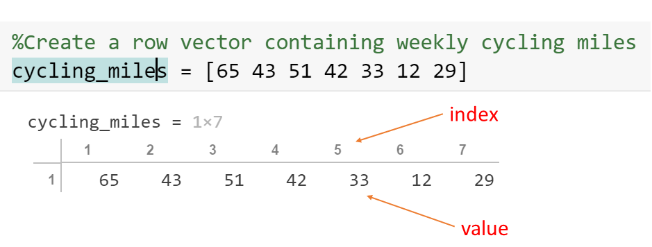
Figure 2.1: Indexes and Values
The row of numbers across the top shows the index of each element of the array, and the bottom row shows the value of each element. For example, the 5th element of the array has the value 33. An index must always be a positive integer between 1 and the length of the array.[1]
The MATLAB syntax for indexing is to put the index in parentheses next to the variable name:
>> week_5_miles = cycling_miles(5)
week_5_miles =
33
It is important to understand that, when we say the value has been extracted from the array, that does not mean that is has been removed from the array. Its value has simply been read and copied to another variable.
Multiple values can be extracted from an array at once by specifying a vector of indices. For example, suppose you want to extract the cycling miles for the first week of each month:
>> miles_1_5 = cycling_miles([1, 5])
miles_1_5 =
65 33
The index vector can also be a range, specified with the colon operator. For example, to extract the miles for the first month:
>> miles_May = cycling_miles (1:4)
miles_May =
65 43 51 42
2.3.1 Extracting Values from a Matrix
Since a matrix has two dimensions, both row and column indices are typically specified. (There is also another way to do it, linear indexing, which will be introduced later.) The value from row 2, column 1 of matrix M2 can be extracted as follows:
>> r2c3 = M2(2, 1)
r2c3 =
4

Figure 2.2: Matrix Indexing
Similarly to 1D arrays, the row or column index can be a vector; this is useful for extracting a submatrix. For example, to extract the 2×2 submatrix from the lower-right corner of M1, the syntax is:
>> submatrix1 = M1(2:3, 2:3)
submatrix1 =
1.5708 3.1416
1.0000 1.0000
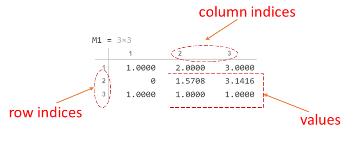
Figure 2.3: Extracting a sub-matrix
A common operation with matrices is to extract an entire row or column. This is done by using a colon as the other index, as in these examples:
>> %Extract row 1 of M2>> M2_r1 = M2(1, :)M2_r1 = 2 10 0>> %Extract column 2 of M1>> M1_c2 = M1 (:, 2)M1_c2 = 2.0000 1.5708 1.00002.3.1.1 Linear Indexing

Figure 2.4: Linear Indexing
>> M1(5:7)
ans =
1.5708 1.0000 3.0000
Notice that the result is stored as a row vector.
Lecture Video 2.3 – Indexing in an Array
Checkpoint 2.3: Indexing
Lecture Video 2.4 – Concatenating Arrays
Checkpoint Questions – Concatenation
2.4 Modifying Elements of Arrays
One or more elements of an array can be assigned values by indexing. In this case, the indexing appears on the left side of the equals sign. For example, suppose that a correction is made to the cycling miles for the first month of May; the array can be modified in MATLAB as follows:
>> miles_May (3) = 61
miles_May =
65 43 61 42
An element can be added to the end of an array using the same method:
>> miles_May (5) = 70
miles_May =
65 43 61 42 70
Since miles_May has only 4 elements before this statement is executed, MATLAB allocates an additional memory location to the array and appends the new value.
Multiple elements of an array can be assigned at once using a set of indices:
>> cycling_miles (8:11) = [44, 49, 53, 40]
cycling_miles =
65 43 51 42 33 12 29 44 49 53 40
When this technique is used, the number of indices on the left-hand side must match the number of values on the right-hand side. The exception is when the right-hand side is a scalar; in that case, all specified elements of the array are assigned to the same value:
>> cycling_miles ([5, 6]) = 55
cycling_miles =
65 43 51 42 55 55 29 44 49 53 40
The syntax is similar for a matrix, except that both row and column indices are provided. For example, to change the row-3, column-2 element of M2 to -1:
>> M2(3, 2) = -1
M2 =
2.0000 10.0000 0
4.0000 6.6667 0
6.0000 -1.0000 0
8.0000 0 0
2.5 Character and String Arrays
Up to this point, we have considered only numerical arrays, but it is often necessary to store text information as well. MATLAB has two distinct ways of storing text information: character arrays and strings. The distinction can be summarized as follows: in a character array, each character can be extracted or modified individually, while a string is an indivisible element.
To illustrate the difference, consider these examples.
>> %This is a string:
>> name_str = "J.E. Toney"
name_str =
"J.E. Toney"
>> %This is a character array
>> name_char = 'J.E. Toney'
name_char =
'J.E. Toney'
>>
Notice that in MATLAB syntax, double quotes (“) indicate a string, while single quotes (‘) indicate a character array. The difference between the two becomes clearer when indexing is used to extract an element:
>> name_char(1)
ans =
'J'
>> name_str(1)
ans =
"J.E. Toney"
>>
In the former case, extracting the first element returns the first character, while in the latter case, it returns the entire string.
Multiple strings can be stored together in a string array. This is the preferred way to store a number of strings, for example, a list of names, when there is no need to access portions of each name. Consider these two examples:
>> names_char = ['Jim', 'Joe', 'Larry', 'Laura']
names_char =
'JimJoeLarryLaura'
>> names_str = ["Jim", "Joe", "Larry", "Laura"]
names_str =
1×4 string array
"Jim" "Joe" "Larry" "Laura"
In the first example, when the names are enclosed in single quotes, the result is a 1×16 character array, with no boundaries between the names. In the second example, when the names are enclosed in double quotes, the result is a 1×4 string array. A single name can be extracted from the string array easily:
>> names_str (3)
ans =
"Larry"
To extract the same name from the character array requires specifying the correct range of indices:
>> names_char(7:11)
ans =
'Larry'
Similarly, indexing can be used to modify one of the names:
>> names_str(3) = "Bobbi"
names_str =
1×4 string array
"Jim" "Joe" "Bobbi" "Laura"
In the case of a character array, the number of characters being replaced must match the number of characters in the new name. In this example, since ‘Larry’ and ‘Bobbi’ have the same number of letters, this can be done without too much trouble:
>> names_char (7:11) = 'Bobbi'
names_char =
'JimJoeBobbiLaura'
Lecture Video 2.5 – Character and String Arrays
Checkpoint 2.4-2.7: Character and String Arrays
2.6 Array Operations
Since MATLAB was created to perform matrix operations efficiently, it has unique built-in capabilities for operating on arrays. Often, a single line of MATLAB code can perform a large set of operations that, in other languages, would be done with a combination of loops and if statements.
2.6.1 Scaling, Offsetting, Adding and Subtracting Arrays
All elements of an array can be multiplied or divided by a scalar value with a single operation. For example, to convert cycling_miles to kilometers:
>> cycling_km = cycling_miles*1.609
cycling_km =
Columns 1 through 9
104.5850 69.1870 82.0590 67.5780 88.4950 88.4950 46.6610 70.7960 78.8410
Columns 10 through 11
85.2770 64.3600
Or to convert the cargo_weights from pounds to kilograms:
>> cargo_kg = cargo_weights / 2.205
cargo_kg =
114.7392 58.5034 39.9093 19.0476 50.3401 12.2449
Similarly, a scalar can be added to or subtracted from an array. For example, to make an array of 2s, start with an array of 1s and add 1:
>> twos = ones(1,8) + 1
twos =
2 2 2 2 2 2 2 2
Or create an array of -1s by subtracting 1 from an array of 0s:
>> minus_ones = zeros(1,6) - 1
minus_ones =
-1 -1 -1 -1 -1 -1
Two or more arrays can be added or subtracted if they have the same dimensions, as in this example, which calculates Willie Stargell’s total number of extra base hits each year by adding the numbers of doubles, triples, and home runs:
>> Stargell_doubles = [3, 11, 19, 25, 30, 18, 15, 31, 18, 26, 28, 43, 37, 42, 20, 12, 18, 19, 10, 4, 4];
>> Stargell_triples = [1, 6, 7, 8, 0, 6, 1, 6, 3, 0, 2, 3, 4, 2, 3, 0, 2, 0, 1, 0, 0];
>> Stargell_homeruns = [3, 0, 11, 32, 28, 13, 20, 22, 25, 44, 33, 48, 31, 29, 24, 20, 33, 27, 21, 11, 0];
>> Stargell_xbase = Stargell_homeruns + Stargell_triples + Stargell_doubles
Stargell_xbase =
7 17 37 65 58 37 36 59 46 70 63 94 72 73 47 32 53 46 32 15 4
The vectors are added element-by-element; the result is a vector with the same dimensions as the vectors being added, where the kth element of the result is determined by adding the kth element of each input vector.
Lecture Video 2.6 – Scalar-Array Operations
2.6.2 Element-wise Operations on Arrays
As discussed above, arrays can be added or subtracted using the usual notation (+ or -). However, multiplying or dividing arrays may require a special notation, depending on what you are trying to accomplish. The reason for this is that there are two different operations that can be described as “multiplying” two arrays. The first is matrix-matrix or matrix-vector multiplication as defined in linear algebra. This book does not cover that type of multiplication. The second is element-by-element multiplication, in which each element of an array is multiplied by the corresponding element of a second array. That is the type of operation that we cover in this book, and it requires a special notation.
To illustrate the difference between the two types of multiplication, consider these two examples:
>> sigma_x * sigma_z
ans =
0 -1
1 0
>> sigma_x .* sigma_z
ans =
0 0
0 0
The first example, which uses the ordinary multiplication operator (*), multiplies the two matrices according to the rules of linear algebra. The second, which uses the element-wise multiplication operator (.*), multiplies the corresponding elements of the two matrices as follows:
>> [sigma_x(1,1) * sigma_z(1,1), sigma_x(1,2)*sigma_z(1,2)
sigma_x(2,1) * sigma_z(2,1), sigma_x(2,2)*sigma_z(2,2)]
ans =
0 0
0 0
This type of operator is also used when dividing two arrays or when raising an array to a power:
>> sigma_x.^2ans = 0 1 1 0>> %fraction of Stargell's extra base hits that were home runs, by year
Stargell_homeruns./Stargell_xbase
ans =
Columns 1 through 9
0.4286 0 0.2973 0.4923 0.4828 0.3514 0.5556 0.3729 0.5435
Columns 10 through 18
0.6286 0.5238 0.5106 0.4306 0.3973 0.5106 0.6250 0.6226 0.5870
Columns 19 through 21
0.6563 0.7333 0
As another example, consider calculating the motion of a particle moving with constant acceleration, according to the formula
[latex]x (t) = \frac{1}{2} a t^2 + v_0 t + x_0[/latex]
Suppose that the calculation is to be performed at 6 values of t, starting at 0 and increasing in one-second increments. The t values can be stored in a vector:
>>t = 0:1:5;
Assuming that variables a, v0, and x0 have already been defined, the corresponding x values can be calculated in one line:
>> x = 1/2*a*t.^2 + v0*t + x0;
The dot is needed when squaring t, since t is an array; it is not needed when multiplying v0 by t, since v0 is a scalar. If the dot is omitted from the squaring operation, this error message will be displayed:
>> x = 1/2*a*t^2 + v0*t + x0;
Error using ^ (line 51)
Incorrect dimensions for raising a matrix to a power. Check that the matrix is square and
the power is a scalar. To perform elementwise matrix powers, use '.^'.
The error occurs because MATLAB interprets t^2 as meaning t*t, in the sense of matrix-vector multiplication, and the dimensions of t are not consistent with that operation.
Lecture Videos 2.7-2.8 – Array Operations
Adding & Subtracting:
Element-Wise Operations
Checkpoint 2.8-2.9: Array Operations
2.6.3 Functions for Arrays
MATLAB, like Excel, has numerous built-in or library functions to perform statistical calculations on arrays. Some of the most common functions that operate on arrays are listed in Table 2.1 below:
Table 2.1 MATLAB Functions for Arrays
| Function | Description |
| mean | statistical average of the values in the array |
| max | highest value in an vector; or higher of two values – works element-wise when applied to two vectors; when applied to a matrix, returns a row vector containing the max of each column by default |
| min | lowest value in an vector; or lower of two values – works element-wise when applied to two vectors; when applied to a matrix, returns a row vector containing the min of each column by default |
| length | number of elements in a vector; when applied to a matrix, the larger of its dimensions |
| size | dimensions of an array, returned as a row vector; e.g. for a MxN matrix the result is [M, N] |
| numel | total number of elements in an array; e.g. for a MxN matrix, the result is M*N |
| median | the statistical median (middle value) of a vector; operates column-wise on a matrix by default |
| mode | the statistical mode (most common value) of a vector; operates column-wise on a matrix by default |
| std | the sample standard deviation of a vector; operates column-wise on a matrix by default |
Uses of the min & max Functions
Many MATLAB built-in functions can operate differently depending on the number and type of inputs that are passed to them. The min and max functions are particularly versatile. The table below shows some of the ways that these functions can be applied with examples.
Table 2.2 : Applications of the max and min functions
| Case | Inputs | Operation | Example |
| 1 | two scalars | higher (lower) of the two | >> max(5,10)
|
| 2 | a vector | highest (lowest) value in the vector | >> max([2,8,4,3,9,-5, 0])
|
| 3 | two vectors | a vector containing the higher (lower) value in each index position | >> max( [2, 4, 6], [1, 5, 3])
|
| 4 | a matrix | the highest (lowest) value in each column | >> max(M1) %(see earlier example)
|
| 5 | a matrix, with 2 as the third argument[2] | the highest (lowest) value in each row | >> max(M2, [], 2) %(see earlier example)
|
| 6 | a matrix, with 'all' as the third argument |
the highest (lowest) value in the entire matrix | >> max (M2, [], 'all')
|
sum and mean, but with those functions the [] is NOT used:>> sum(M1,2)
ans =
6.0000
4.7124
3.0000
>> mean(M2, 'all')
ans =
3.3333
>> [max_hr, max_yr] = max(Stargell_homeruns)
max_hr =
48
max_yr =
12
This tells us that the largest number of home runs that Willie Stargell hit in a year was 48, and that number is in the 12th position of the array. Given that the data are in reverse chronological order, and Stargell played from 1962 to 1982, a vector of years can be defined, and the variable max_yr can be used as an index to extract the year in which he had his maximum home run production:
>> years = 1982:-1:1962;
>> years(max_yr)
ans =
1971
Lecture Video 2.9 – Statistical Functions for Arrays
Checkpoint 2.10-2.11: Built-in Functions for Arrays
2.7 Mathworks Resources
2.8 Problems
-
The company Buckeye Products, Inc. is forecasting its cash flow for the upcoming year. Their sales are mostly made on account, meaning that the cash is not received until up to 2 months after the sale. From past experience, they know that they can reliably assume that
- 20 % of payments will be received in the same month as the sale
- 70 % of payments will be received in the month following the sale
- 10 % of payments will be received two months following the sale
The company plans to introduce a new product on January 1 of next year. They have forecast the sales revenues from this product for each month. Given the sales forecast as a 1×12 array,(a) Calculate the expected cash received for this product in each month of next year. Store the results in a row vector.(b) Determine the month in which the cash received is maximum, and print out that result with an appropriate message.You can test your code with the following values for the month-by-month sales forecast:[latex]\\[/latex]sales = [400000, 600000, 800000, 70000, 650000, 625000, 750000, 800000, 775000, 725000, 650000, 600000][latex]\\[/latex]answer: The maximum cash received should be 700000 in September[latex]\\[/latex]
HINT: To avoid the need for a loop or if statement (which are covered in a later chapter), create two additional vectors: sales_1 and sales_2, with the sales figures shifted by one or two positions and zeros added to the beginning. You can then calculate then monthly cash received as a weighted sum of the 3 vectors.
[latex]\\[/latex]
-
Present Value of an AnnuityRetirees often purchase an annuity to give them stable income for a number of years. In this type of investment, the recipient gives the provider (usually an insurance company) a lump sum and receives equal payments for a specified number of years.The “present value” of an annuity is the lump-sum amount that is deemed to be economically equivalent to the annual payments, assuming a certain rate of interest. For example, if the annuity pays $1,000 /year for 20 years, the present value would be something LESS than $20,000, because money received in the future is valued less than money received today.The present value (assuming annual payments) is defined as follows:[latex]\\[/latex][latex]PV = A (\frac{1}{1+r} + \frac{1}{(1+r)^2} + ... )[/latex][latex]\\[/latex]where A is the amount of the annual payments and r is the interest rate expressed as a fraction. (So if the interest rate is 10 %, r = 0.10)[latex]\\[/latex]In more compact notation, this can be written:[latex]\\[/latex][latex]PV = A\Sigma_{k=1}^n \frac{1}{(1+r)^k}[/latex] where n is the number of years over which the annuity pays out.[latex]\\[/latex]Calculate the present value (PV), given values for A, n and r.To test your code, use A = $1000, interest rate = 20 %, and n = 5 years. Answer: $2991.[latex]\\[/latex]
-
Moments and Products of Inertia
Given the dimensions of a rectangular solid, a, b, and c, the inertia tensor for rotation about a corner of the body is as follows for a solid block of density ρ:[latex]I= \left( \begin{array}{ccc} I_{xx} & I_{xy} & I_{xz} \\ I_{xy} & I_{yy} & I_{yz} \\ I_{xz} & I_{yz} & I_{zz} \end{array} \right)[/latex]where[latex]I_{xx} = \frac{\rho V}{3}(b^2+a^2)[/latex][latex]I_{yy} = \frac{\rho V}{3}(c^2+a^2)[/latex][latex]I_{zz} = \frac{\rho V}{3}(b^2+c^2)[/latex][latex]I_{xy} = \frac{\rho V}{4}cb[/latex][latex]I_{xz} = \frac{\rho V}{4}ac[/latex][latex]I_{yz} = \frac{\rho V}{4}ab[/latex][latex]V = a b c[/latex]Given values of a, b, c, and ρ, calculate the matrix [latex]I[/latex].To test your code, use a = 2.5069, b = 2.2455, c = 14.03, ρ = 3.451. Take the sum of the entire matrix; the result should be 47678.[latex]\\[/latex] - Tic-Tac-Toe Grid

5. Loading, Displaying, and Modifying a Grey-Scale Image
In MATLAB, a grey-scale image is just a matrix of numbers between 0 and 255 (0 = black, 255 = white; other values are shades of grey). In this problem, you will experiment with modifying the characteristics of grey-scale image by simple arithmetic operations. (Much more sophisticated image manipulation can be performed with the Image Processing Toolbox.)
a) Download this file: puppy.mat and move it to your MATLAB directory. You can load and display the image with the following commands, either at the command line or in a script:
load pupply %creates an image matrix called puppy in the workspace
imshow(puppy) %displays the image in a figure window
b) Make a copy of the image by adding 50 to the matrix and assigning it to a new variable (puppy1, for example). Show the modified image – it should be brighter than the original
c) The contrast of the image can be increased by applying a nonlinear scaling of this form:
M’ = a M2 + b M
where b < 1 and a = (1 – b)/255. Make a third copy of the puppy image by applying this scaling to the original matrix, using b = 0.5 and a = 0.5/255. Show the third image – it should have higher contrast than the original.
SPECIAL COMPUTATIONAL NOTE: Because grey-scale images only take the values 0 through 255, they are stored in a data type called uint8 (unsigned 8-bit integer). For the scaling calculation to work properly, the matrix must be converted to a single-precision integer format prior to the calculation, then BACK to uint8 format after the calculation. An example sequence is:
>> y = single (puppy)
>> z = … %perform the scaling calculation
>> puppy2 = uint8(z)
d) Create a 4th copy of the image that only shows the most prominent edges (an outline view), by doing the following:
-
- Subtract the 3rd (contrast-enhanced) image from the original one. IMPORTANT, because images are an unsigned data type (they cannot have negative values), the subtraction must be done in this order: original image MINUS modified image
- Multiply the original image (element-wise) by the difference calculated in i.
Show the last image. It should show a dark outline of the figure.
6. In the Braille alphabet, each letter is represented by a 3×2 array of dots/white space. For example, the letters ‘c’, ‘a’, and ‘t’ are


a) Create three 3×2 matrices representing c, a, and t, with a 1 for each black dot and a 0 for each white space.
b) Concatenate the three matrices into a 3×6 matrix representing “cat”. The resulting matrix should be:
[latex]\begin{bmatrix}1 &1 &1 &0 &0 &1\\0 &0 &0 &0 &1 &1\\0 &0 &0 &0 &1 &0\end{bmatrix}[/latex]
7. Rotation Matrices
theta = rand()*2*pi;(b) Create the three matrices, R_x, R_y, and R_z.
epsilon0 = 8.85e-12;%values of the chargesq = randi([-10, 10], 1, 8)/1e6;%x-and y-coordinates of the chargesx= randi([-10, 10], 1, 8);y= randi([-10, 10], 1, 8);[latex]\\[/latex]
[latex]\\[/latex]
declaration = 'We hold these truths to be self-evident, that all men are created equal, that they are endowed, by their Creator, with certain unalienable Rights, that among these are Life, Liberty, and the pursuit of Happiness. That to secure these rights, Governments are instituted among Men, deriving their just powers from the consent of the governed, That whenever any Form of Government becomes destructive of these ends, it is the Right of the People to alter or abolish it, and to institute new Government, laying its foundation on such principles, and organizing its powers in such form, as to them shall seem most likely to effect their Safety and Happiness. Prudence, indeed, will dictate that Governments long established should not be changed for light and transient causes; and accordingly all experience hath shewn, that mankind are more disposed to suffer, while evils are sufferable, than to right themselves by abolishing the forms to which they are accustomed. But when a long train of abuses and usurpations, pursuing invariably the same Object, evinces a design to reduce them under absolute Despotism, it is their right, it is their duty, to throw off such Government, and to provide new Guards for their future security.'extractBetween and strrep in this problem. Since declaration is a character array, not a string, the problem can be done with simple indexing.
%Generate 5 random forcesF = randi([100, 1000], 1,5);r = rand(1, 5);theta = randi([0, 180], 1,5);[latex]Mi = F_i r_i sin \theta_i[/latex]
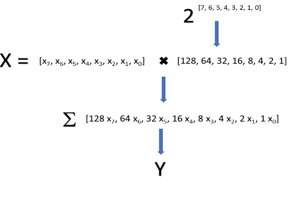
X = randi([0,1], 1, 8)BaP = 0.2 * (0.75+rand()/2);BaA = 0.52 * (0.75+rand()/2);BbF = 0.09 * (0.75+rand()/2);BkF = 47 * (0.75+rand()/2);Chry = 98 * (0.75+rand()/2);DahA = 0.1 * (0.75+rand()/2);I123P = 0.5 * (0.75+rand()/2);
mission_statement = ['We must all efficiently Operationalize our strategies',...'Invest in world-class technology',...'And leverage our core competencies',...'In order to holistically administrate',...'Exceptional synergy',...'We''ll set a brand trajectory',...'Using management''s philosophy',...'Advance our market share vis-à-vis',...'Our proven methodology',...'With strong commitment to quality',...'Effectively enhancing corporate synergy',...'Transitioning our company',...'By awareness of functionality',...'Promoting viability',...'Providing our supply chain with diversity',...'We will distill our identity',...'Through client-centric solutions',...'And synergy'];[latex]\\[/latex]
Find an error? Have a suggestion for improvement? Please submit this survey.
