3 Input-Output & Plotting
To be really useful, a computer program must interact with the user. That means allowing the user to enter information and displaying results to the user, either in numerical, text, or graphical form. A later chapter will cover graphical user interface (GUI) programming; this chapter covers simple methods for numerical and text input/ouput and graphical display of data.
3.1 User Input
The simplest way to request information from the user of a MATLAB program is with the function, input(). This function displays a prompt to the command window asking the user to enter a value and waits for the user to respond. The value entered by the user is stored in a variable. The basic form of the call to the input function is
variable_name = input (prompt)
For example, this line requests and stores the user's age:
>> user_age = input ('Please enter your age: ')
Please enter your age: 29
user_age =
29
In addition to numerical values, input can also accept text input. When the user is expected to enter a string rather than a number, a second argument, 's', is included, as in this example:
>> user_name = input ('Please enter your name: ', 's')Please enter your name: Brutususer_name = 'Brutus'>> name = input ('Please enter your name: ')Please enter your name: BrutusError using inputUnrecognized function or variable 'Brutus'.Please enter your name: Please enter your name: 'Brutus'
name =
'Brutus'
but it is better to use the 's' argument for the user's convenience.
>> quiz_scores = input ('Enter the student''s quiz scores in [ ]: ')
Enter the student's quiz scores in [ ]: [79, 83, 91, 85]
quiz_scores =
79 83 91 85
>> quiz_scores = input ('Enter the student''s quiz scores in [ ]: ')
Enter the student's quiz scores in [ ]: [79; 83; 91; 85]
quiz_scores =
79
83
91
85
>> user_matrix = input ('Enter a 2x2 matrix in [ ]: ')
Enter a 2x2 matrix in [ ]: [3 2; 1 4]
user_matrix =
3 2
1 4
Checkpoint 3.1-3.2: input
3.2 Command-line Output using disp
As discussed in Chapter 1, mixed text-numerical output can be displayed to the command window using the disp() function. The text and numerical components can be joined into a single string using +, as in this example:
>> disp("I am " + my_age + " years old")
I am 29 years old
Of course, the variable my_age must have already been defined. disp () does not have formatting capability, but the number of decimal places in a floating-point number can be controlled using the round() function:
>> BMI = 703*200/70^2
BMI =
28.6939
>> disp("My body mass index is " + round(BMI,1)) %display BMI with 1 decimal place
My body mass index is 28.7
Checkpoint 3.3 - 3.4: disp
3.3 Formatted Output using fprintf
The fprintf() function provides more control over the formatting of command-line output. It also allows writing to a text file (the first f stands for "file", and the second one for "formatted"). The basic syntax of fprintf for writing to the command window is
>> fprintf('String including format descriptors and special characters', variable_list)
A format descriptor can be thought of as a placeholder; it can be interpreted as, "a value to be supplied later - in the variable list that follows." The example above, using disp() to print "My age is...", can be implemented with fprintf() as follows:
>> fprintf('My age is %i', my_age)
The %i is a format descriptor that specifies an integer value. If the value being printed is a floating-point number (i.e. a number with a decimal point), the %f format descriptor is used:
>> fprintf('My body mass index is %f', BMI)
My body mass index is 28.693878
By default, the number is displayed with unreasonably high precision. To control the number of decimal places, the format descriptor is written as %.nf, where n is the desired number of digits after the decimal point. The example above, using disp() to display the body mass index with 1 decimal place, is implemented with fprintf() as follows:
>> fprintf('My body mass index is %.1f', BMI) %display BMI with 1 decimal place
My body mass index is 28.7
Other commonly used format descriptors are %s = string, %c = character, and %e = number in scientific notation. To print the values of multiple variables intermixed with text, a format descriptor is used for each variable, and the variables are listed in the same order. For example (assuming that a variable name has already been defined):
>> fprintf('My name is %s, I am %i yrs old, and my BMI is %.1f', name, my_age, BMI)
My name is Jim, I am 29 yrs old, and my BMI is 28.7
3.3.1 Special Characters
Certain special characters, such as tab and newline, can be included in the string; often they are preceded by a backslash (\). Some of the most commonly used special characters are:
\n newline
\t tab
\xN unicode, where N is the hexadecimal code of the character
\\ backslash
%% percent symbol
It is important to remember that in a script, unlike disp(), fprintf() will not go to a new line until it encounters a \n character. Notice the difference in these two examples:
%1. newline character not included
fprintf('My name is %s', name)
fprintf('My age is %i', my_age)
My name is JimMy age is 29>>
%2. newline character included
fprintf('My name is %s\n', name)
fprintf('My age is %i\n', my_age)
My name is Jim
My age is 29
>>
It is best to get into the habit of always including a \n at the end of the string, except in the special cases when it is not wanted.
3.3.2 Field Width
To facilitate alignment for printing tables, the width of each number or text field can be controlled by putting the number of spaces allocated to the value immediately after the % in the format descriptor. For example, consider the difference in these two lines (03C0 is the hexadecimal unicode for [latex]\pi[/latex]):
fprintf('The value of \x03C0 is %.2f\n', pi)
fprintf('The value of \x03C0 is %8.2f\n', pi)
The value of π is 3.14
The value of π is 3.14
>>
In the first case, no field width is specified, so the minimum necessary number of spaces (4) is used to represent the number. In the second case, a field with of 8 spaces is specified, so the number is padded with 4 leading blanks.
The example below shows how these features can be used to print a right-justified table. (Note: for convenience, this example uses a for loop, which is covered in Chapter 6.)
Lecture Video 3.1 - Basic Input & Output
You can download the Live Script
Checkpoint 3.5: fprintf
3.4 Plotting
MATLAB has a wide range of capabilities for graphical presentation of data. This section focuses exclusively on line and scatter plots. See the MATLAB documentation or other online resources for coverage of bar charts, pie charts, contour and surface plots, etc.
The function to create a line or scatter plot is plot(). The most basic call to this function is
>> plot (x_data, y_data)
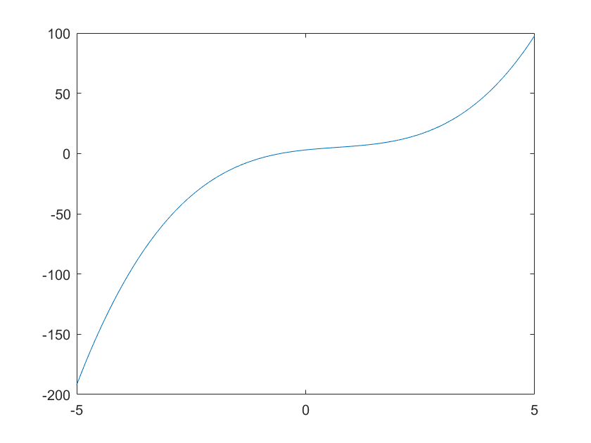
This function creates a figure window containing the plot as in this example:
>> x = -5:0.1:5;
>> y = x.^3 - 2*x.^2 + 4*x +3;
>> plot(x,y)
To annotate the plot, the functions xlabel(), ylabel(), and title() are used:
>> xlabel('x values')
>> ylabel('y values')
>> title('x^3 - 2x^2 + 4x +3')
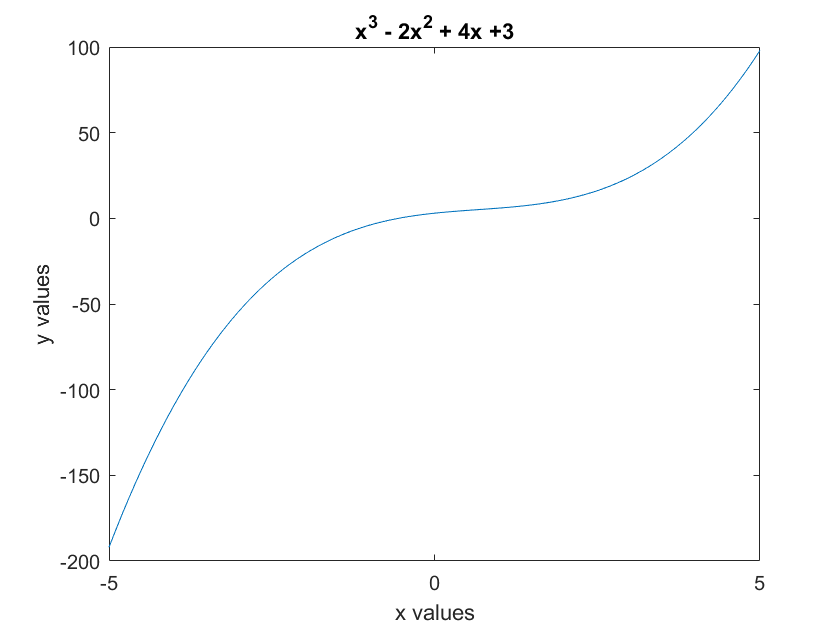
Notice that MATLAB the ^ character as meaning exponentiation and writes the following number as a superscript.
A second data series can be added to the same plot by executing the command:
>> hold on
This tells MATLAB to overlay the next plot onto the existing one, instead of overwriting it. A plot with multiple data series should have a legend, which is added using the legend() function.
> z = -0.5*x.^4 + x.^3 - 2*x.^2 + 4*x +3;
>> hold on
>> plot(x, z)
>> legend('3rd-order', '4th-order')
>> title('Polynomials')
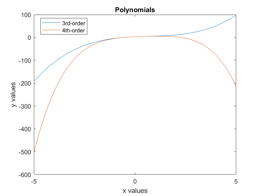
Notice that by default MATLAB represents each data series by a different color of solid line. The appearance of the plot - solid vs. dashed or dotted lines, line colors, markers - can be changed using control strings. For example, if the above plot is going to be printed in black-and-white, it is better to use different line styles rather than colors. This example plots both data series at once - without using hold on - one as a solid black line and the other as a dashed black line:
>> plot(x, y, 'k-', x, z, 'k--')
>> xlabel('x values')
>> ylabel('y values')
>> title('Polynomials')
>> legend('3rd-order', '4th-order', 'Location', 'Northwest')
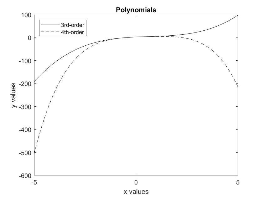
In this example, the legend position was specified as 'Northwest', which means the upper-left corner. (The default is upper-right, which in this case would have covered part of the plot.) The control character for black is 'k', since 'b' is used for blue.
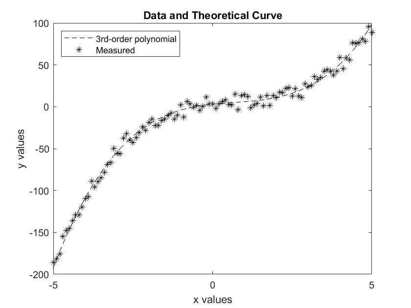
Another option is to represent a data series by markers instead of (or in addition to) a line. The usual practice is to use markers for experimental data and lines for theoretical curves. Suppose that there is an array of experimental results, y_exp, for a quantity that is described theoretically by the 3rd-order polynomial shown above. To plot the experimental and theoretical results on the same graph:
>> plot(x, y, 'k--', x, y_exp, 'k*')
>> xlabel('x values')
>> ylabel('y values')
>> title('Data and Theoretical Curve')
>> legend('3rd-order polynomial', 'Measured', 'Location', 'Northwest')
A list of control the characters for colors, line styles and marker types can be found in the MATLAB documentation.
3.4.1 Sub-Plots
There are cases in which it is useful to include multiple plots in the same figure, but not on the same axes. For example, in a mechanics simulation, there may be plots of acceleration, velocity, and position, but since these quantities have different dimensions, it is not sensible to put them on the same axes.
One way of including multiple plots on separate axes in a single figure is with subplots. [1] To include multiple plots as subplots in a single figure, the subplot() function is called prior to each plot() call. The format of the call is
>>subplot(rows, columns, index)
where rows and columns specify the arrangement of the subplots, and index specifies which subplot is currently being plotted. For example
>>subplot(3, 1, 1)
>>plot (x,y)
indicates that a 3x1 subplot - 3 plots arranged vertically - is being created, and y vs. x is plotted in the first (top) subplot.
An example of using a 3x1 subplot to graph results of a mechanics simulation is given below.
%{Plot altitude, velocity, and acceleration from a sky-diving simulation in a 3x1 subplot. Since the plots share a common time axis, only use an xlabel for the bottom plot. Place a %title only on the top plot.%}subplot(3,1,1)plot(t,y)ylabel('Altitude (m)')title ('Sky-Diving Simulation')subplot(3,1,2)plot(t,v)ylabel('Velocity (m/s)')subplot(3,1,3)plot(t,a)ylabel('Acceleration (m/s^2)')xlabel('Time (s)')
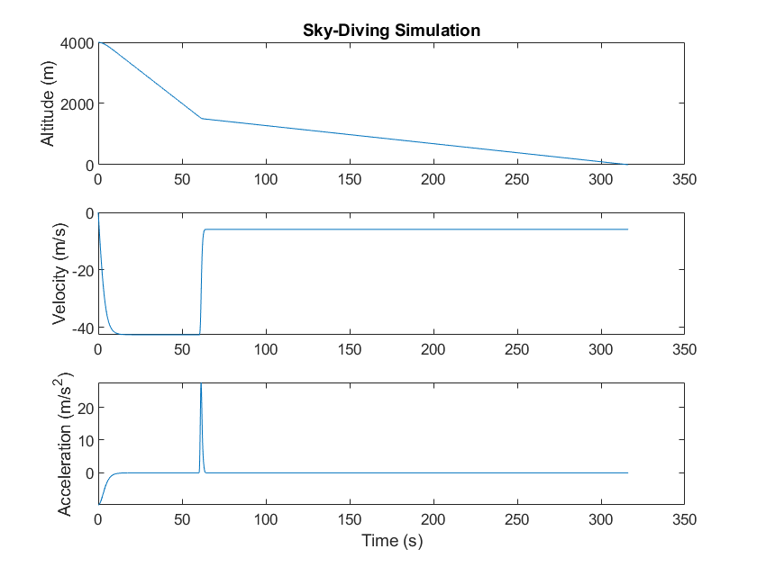
A legend is not needed in this case, since each subplot has only one data series.
In the case of a 2D arrangement of subplots, the tiles are numbered row-by-row; for example, in a 2x2 subplot, the tile numbering is as follows:
| 1 | 2 |
| 3 | 4 |
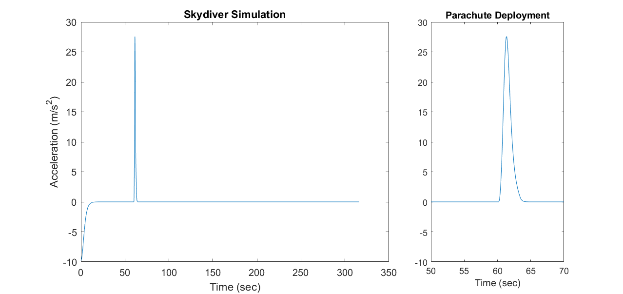
Multiple tiles can be allocated for a single plot, as in the following example:
%Plot acceleration of skydiver
%First plot takes two tiles
subplot (1,3,1:2)
plot(t, a)
xlabel('Time (sec)')
ylabel ('Acceleration (m/s^2)')
title('Skydiver Simulation')
%second plot zooms in around parachute deployment
%only takes one tile
subplot(1,3,3)
plot(t, a)
xlabel('Time (sec)')
axis([50,70, -10,30])
title('Parachute Deployment')
3.4.2 Double-y Graphs
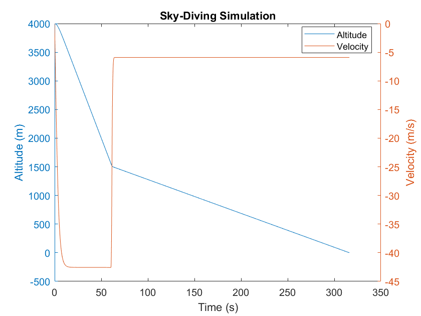
Another way to place multiple plots on different axes in the same graph is a double-y-axis graph. In this method, the plots share a common x-axis but use different y-axes - one on the left of the graph and one on the right. To specify which y-axis each plot uses, the command yyaxis left and yyaxis right are used.
The example below plots the altitude and velocity from the previous example on a double-y graph.
%Plot altitude and velocity on separate y-axes
yyaxis left %not really necessary, since left is the default
plot(t,y)
ylabel('Altitude (m)')
yyaxis right
plot(t,v)
ylabel('Velocity (m/s)')
xlabel('Time (s)')
title ('Sky-Diving Simulation')
Lecture Videos 3.2 - 3.4 - Plotting
Checkpoint 3.6 - 3.8: Plotting
3.5 Mathworks Resources
3.6 Problems
- Harmonic Analysis
A fundamental technique of engineering analysis is Fourier decomposition - representing a periodic function as a sum of sine or cosine functions at multiples of the fundamental frequency. For example, a periodic triangular wave can be written as a sum of cosines. In this problem you will create a plot to show how a triangle wave function can be approximated by a sum of cosines, and how the approximation becomes more accurate as more terms are included in the sum.
The underlying theory is somewhat complicated, but for this problem only these two equations are needed:
[latex]x_T(t) = a_0 + \sum_{n=1}^{+\infty}a_n\ cos({n\ \omega_0\ t})[/latex]
[latex]a_n = 4A\frac{1-(-1)^n}{\pi^2n^2},\ n\ odd[/latex]
[latex]a_n = 0,\ n\ even[/latex]
TERMINOLOGY NOTE: The n = 1 term is called the "fundamental", and the other terms are called "harmonics"; the third harmonic has a frequency of [latex]\omega_3 = 3\ \omega_0[/latex]
Using this cosine series, calculate the first four non-zero terms of the series over the domain [latex]t = [-2\pi, 2\pi], a_0 = 0, \omega_0 = 1, and A = 1[/latex]. Choose the step size so that you get a smooth plot. Create one graph containing the plots of the following vs. t:
a. The fundamental term (n = 1)
b. The sum of the first two terms (fundamental plus 3rd harmonic (n=3)
c. The sum of the first four terms (fundamental, 3rd, 5th, and 7th harmonics)
d. The exact function , which can be calculated using the MATLAB library function sawtooth() as follows:
x_exact = sawtooth(t+pi, 1/2);
For more technical details and to verify the correctness of your plot, refer to this website. (Scroll down to the Even Triangle Wave section.)
2. Plotting Conic Sections
You may have learned in pre-calculus that circles, ellipses, parabolas and hyperbolas are all generated by the intersection of a plane with the surface of a cone – i.e. conic sections. The general form of the equation for a conic section in the xy plane is
[latex]A\ x^2 + B\ xy + C\ y^2 + D\ x + E\ y + F = 0[/latex]
In this problem you will plot a conic section based on a set of coefficients input by the user.
In your script:
a) use the input() function to prompt the user to enter the coefficients A through F as an array.
b) Extract the elements of the input array into separate variables, A, B, C, etc. (No error checking is
required – you may assume that the user entered an array of 6 numbers.)
c) Create a vector of x values ranging from -10 to +10 in steps of 0.1
d) Taking x as the independent variable, calculate the two branches of the curve from the quadratic
formula as follows:
[latex]y_1 = \frac{-(Bx+E) + sqrt{(Bx+E)^2-4C(Ax^2+Dx+F)}}{2C}[/latex]
[latex]y_2 = \frac{-(Bx+E) - sqrt{(Bx+E)^2-4C(Ax^2+Dx+F)}}{2C}[/latex]
e) Plot y1 vs. x and y2 vs. x on the same graph, using the same line style and line color for both.
f) Use the xline() and yline() functions with a line width of 2 to create x- and y-axis lines. (See the MATLAB help for details.)
g) Use the command axis equal to set the aspect ratio of the plot to 1, so that the shape of the
conic sections is not distorted.
There may be extraneous lines outside the boundaries of the conic section, but don't worry about that for now. A problem in a subsequent chapter will discuss how to eliminate them. An example of how the plot should look with coefficients [1, 2, 3, 4, 5, 6] (an ellipse) is shown below.
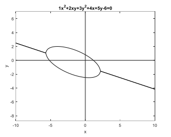
Here are some other test cases that you can try:
i. Parabola: [1, 6, 9, 8, 1, 4]
ii. Circle: [1, 0, 1, 0, 0, -36]
iii. Ellipse: [1, -2, 3, 0, 0, -36]
iv. Hyperbola: [1, 4, -2, 1, 1, 1]
3. Using Subplots
After completing the previous problem, run it on test cases i through iv, and plot the four curves in a single figure as a 2x2 subplot.
Find an error? Have a suggestion for improvement? Please submit this survey.
- NOTE: In the latest releases of MATLAB,
subplothas been supplanted bytiledlayout,which according to Mathworks, "provides more control over labels and spacing thansubplot." This chapter has not yet been updated to reflect this change. As of 2025,subplotis still available for use. ↵
