1 Calculating and Scripting with MATLAB
The easiest way to start learning to use MATLAB is through the command line interface. When the MATLAB environment opens, it looks something like this:
![]()
Figure 1.1: The MATLAB environment
The large area in the middle is the command window, where individual lines of MATLAB code can be entered, and the results are displayed.
What makes MATLAB especially convenient for newcomers to programming is that it is an “interpreted” language, like Python, rather than a “compiled” one, like C or Java. The difference is that a program in a compiled language must be processed in two steps: first it is converted to “machine code”, a low-level representation of the program that can be executed directly by the CPU, then it is executed. An interpreted language, on the other hand, is converted to machine code at the same time that it is run (in a simplified way of looking at it). As an analogy, imagine that you want to understand a speech given in a foreign language that you don’t understand. There are two approaches: you could have the speech translated (compiled) into your native language and read it later, or you could have it interpreted in real time, line-by-line. A C or Java compiler is like a translator, while the MATLAB (or Python) environment is like a simultaneous interpreter.
The reason that interpreted languages are a bit easier for novices to learn is that they make it possible try code out one line at a time. For example, this line of MATLAB code can be entered at the command prompt, divorced from any other context, and the answer is presented immediately (try it!):
>> seconds_per_year = 365 * 24 * 60 * 60
seconds_per_year =
31536000
>>
The >> is the command prompt that appears in the MATLAB command window, not something that the user types. The rest of the first line is a MATLAB “statement”, “instruction”, or “command” – the terms are used more-or-less interchangeably – that tells the interpreter to perform a calculation and store the result. The second and third lines are MATLAB’s presentation of the result of the calculation. The * symbol means multiplication, so this statement multiplies 365 (day/year) x 24 (hrs/day) x 60 (minutes/hr) x 60 (seconds / minute). Notice that there is no indication of units in the instruction – MATLAB has no innate understanding of dimensions or units. The result is stored in a “variable” called seconds_per_year – more about this concept in the next section.
The objective of programming is to arrange a sequence of instructions in advance, then execute them in rapid succession, but we will leave that for a later section.
1.1 Storing Information – Variables
An advantage of using a computer to perform complex calculations is that it enables dividing the calculation into steps. The results of each step can be stored for use in subsequent steps. A variable is just a way to refer to a value (or as we will see in the next chapter, set of values) that is stored in computer memory. In the example above, seconds_per_year is a name that is attached to a location in the computer’s memory that stores the value 315360000.
The whole point of a “variable” is that it can change. Suppose it occurs to you that a year is not really 365 days, but 365 1/4 days. You can re-do the calculation above and get an updated result:
>> seconds_per_year = 365.25 * 24 * 60 * 60
seconds_per_year =
31557600
The value of the variable seconds_per_year has been changed, but it still refers to the same location in the computer’s memory. The previous value that was stored there has been overwritten – it is no longer in the computer’s memory.
A statement like this that has a variable name followed by an equals sign (=) and an expression (which could simply be a number) is called an assignment statement. It means, “store the value of the expression on the right of the = in the variable given on the left.” Unlike in mathematics, it is not a statement that the two things are equal – it is an operation that makes the variable equal to the given expression. Beginning programmers are often confused by a statement like this:
>> x = x + 1
How can x be equal to x + 1? Mathematically, it cannot. What this statement is doing is taking the current value of x (based on whatever operations were performed previously), adding 1 to it, and storing that back in the variable x.
Checkpoint 1.1
The current value of a variable can be examined two ways. First, if the name of the variable is typed at the command line, MATLAB displays its value:
>> seconds_per_year
seconds_per_year =
31557600
Second, the variable can be examined in the “workspace”, which is the area in the right of Figure 1.1. After the revised calculation is performed, it appears like this:
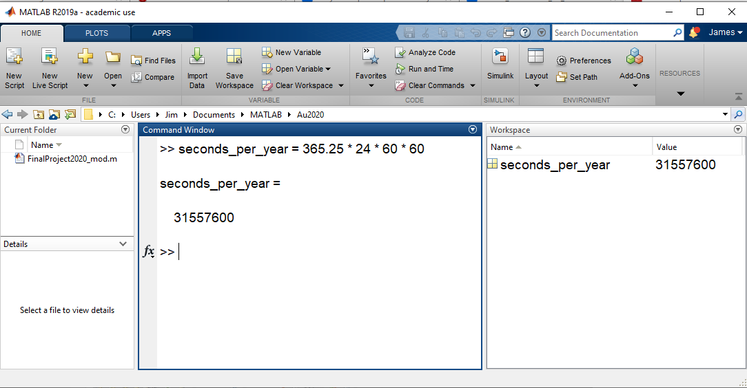
Figure 1.2: Seeing the value of a variable in the workspace
On the right, all variables stored in memory are listed with their current values.
The purpose of storing values in memory is so that they can be used in subsequent steps of a calculation. To illustrate the point, suppose that you want to calculate the speed of light in miles per year, given that you know its value in S.I. units (299,792,458 m/s). You could first calculate the number of meters in a mile, given that 1 mile = 5280 feet, and 3.28 feet = 1 meter:
>> meters_per_mile = 5280/3.28
meters_per_mile =
1.6098e+03
Notice that the result was displayed in scientific (or exponential) notation. e+03 means “times 10 to the 3rd power.”
Next, the results from the two previous steps can be used to calculate the end result:
>> c_miles_per_year = 2.99792458e8 * seconds_per_year / meters_per_mile
c_miles_per_year =
5.8771e+12
Here the division operator (/) has been used. Once this series of calculation has been performed, the workspace window looks like this:
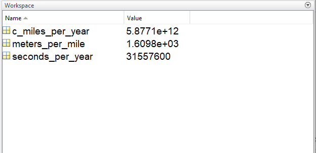
Figure 1.3: A list of variables in the workspace
1.1.1 Valid Variable Names
The rules for variable names are:
- can be 1 to 63 characters long
- can contain letters, numbers, and the underscore (_), but no other special characters
- must begin with a letter
- letters can be upper or lowercase, but variable name is case sensitive – for example,
avg_scoreis a different variable name thanAvg_score.
Variable names should be chosen to help a reader of the program understand what the program is doing. For instance, a variable storing the number of students could be called num_students, numberOfStudents, etc., but it should not be called N, which gives little indication of what the variable represents.
Underscores are often used as separators to make multi-word variable names easier to read. For example, average_score is preferable to averagescore. Another convention that many programmers use is capitalizing every word but the first, e.g. averageScore or finalExamScore. (It is legal to capitalize the first word as well, but the convention is not to do so.)[1]
Checkpoint 1.2
1.2 Performing Arithmetic Calculations
Two of the basic arithmetic operators (* and /) have been demonstrated in previous examples. The remaining operators are:
+ addition
- subtraction
^ exponentiation (raising to a power)
Parentheses can be used to group terms as needed. The standard rules for order of operation apply:
- parentheses
- exponentiation
- multiplication & division
- addition & subtraction
When there are multiple operations of equal precedence, they are performed from left to right.
Checkpoint 1.3 – 1.4
1.3 Performing Calculations Using Built-in or Library Functions
There are many routine calculations in engineering that require special functions – e.g. trigonometric functions, logarithms, statistics, etc. MATLAB includes functions to perform these operations – they are called built-in or library functions, depending on how they are implemented.
To use a MATLAB function, the name of the function is given, with its argument(s) (the value(s) on which it is operating) enclosed in parentheses. For example:
square_root_of_2 = sqrt (2)square_root_of_2 =1.4142Here sqrt ( ) is the MATLAB built-in function that calculates the square root. The argument does not have to be a simple number – it can be a complex expression or a variable, as well. For example, a two-line sequence to calculate the sine of 30 degrees could be:
>> theta = pi/6
theta =>> sine_of_theta = sin (theta)sine_of_theta =0.5000sin – there is no ‘e’. Second, it takes its argument in radians, not degrees – pi/6 radians is equivalent to 30 degrees. There are also functions to calculate the cosine and tangent, called cos and tan, respectively.sind, cosd, and tand. Thus the following lines of code all give the same result:>> cos(pi/3) / sin (pi/3)
ans =>> cosd (60) / sind (60)
ans =>> 1 / tan(pi/3)
ans =>> 1 / tand (60)ans =0.5774ans (short for ‘answer’).| Function Name | Operation |
| sin, cos, tan | sine, cosine or tangent of number in radians |
| sind, cosd, tand | sine cosine, or tangent of angle in degrees |
| log | NATURAL logarithm |
| log10 | BASE 10 logarithm |
| exp | e (base of natural log) raised to a power |
| asin, acos, atan, asind, acosd, atand | inverse trigonometric functions (arcsine, etc.) |
| sqrt | square root |
| round | rounds off a number using the standard convention |
| ceil | rounds a number UP to the next higher integer (short for “ceiling”) |
| floor | rounds a number DOWN to the next lower integer |
Checkpoint 1.5
One of the problems in the previous checkpoint question actually produces a surprising answer when executed in MATLAB. Try this:
>> sin (pi)
Did you get the answer you expected? Always keep in mind that computers perform calculations with finite precision, so mathematical operations may not produce the exact answer that you expect.
1.4 Beyond the Command Line – Scripting
The transition from using MATLAB to programming in MATLAB occurs when you move away from the command line and begin assembling sequences of instructions using the editor. The simplest kinds of programs, involving a linear sequence of operations in a single file, are sometimes called “scripts.” There is no rigid distinction between “script” and “program”; generally, any program that does not use user-defined functions (discussed beginning in Chapter 4) may be thought of as a script.
To open the editor, click the New Script button in the upper left on the home tab:
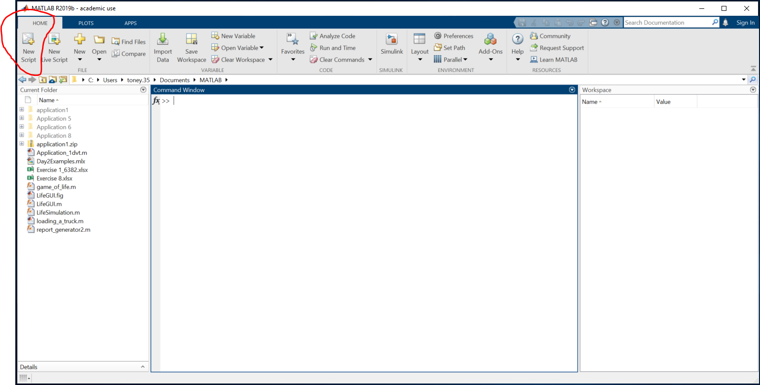
Figure 1.3: Creating a new script
This will open the editor window:
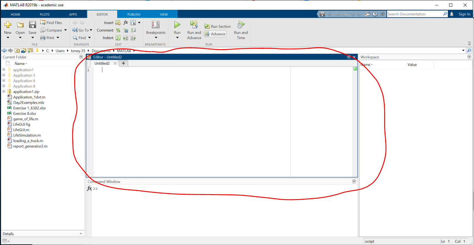
Figure 1.4: The editor window
Any sequence of MATLAB instructions can be entered in the editor and saved for later execution.
As an example, consider calculating successive approximations of [latex]\pi[/latex] based on the Leibniz formula:
[latex]\pi = 4 (1 - \frac{1}{3} + \frac{1}{5} - \frac{1}{7} +\frac{1}{9} + ...)[/latex]
Suppose we want to calculate the first nine approximations to get an idea of how fast this series converges. The most simplistic way of performing the calculations, using the limited set of MATLAB capabilities that we have introduced so far, is this:
%Calculate successive approximations of pi using the Leibniz formula
pi1 = 4
pi2 = pi1 - 4/3
pi3 = pi2 + 4/5
pi4 = pi3 - 4/7
pi5 = pi4 + 4/9
pi6 = pi5 - 4/11
pi7 = pi6 + 4/13
pi8 = pi7 - 4/15
pi9 = pi8 + 4/17
The first line, beginning with a %, is a comment. It performs no function in the program; it is only there to document the program, so that a person reading the code will understand what it does.
After these lines are entered in the editor, the file must be saved under a suitable name. A MATLAB code file has the extension .m, so a suitable name for this file might be Leibniz_pi.m. WARNING: MATLAB file names can only contain letters, numbers and underscores, just like variable names. Never put a blank space in a file name. Once the file has been saved it can be execute by clicking the Run button (the green arrow in the middle at the top) or by typing the filename at the command prompt. The result of each operation will be displayed to the command window. Here the windows have been rearranged so that the editor and command windows are side-by-side for better visibility.
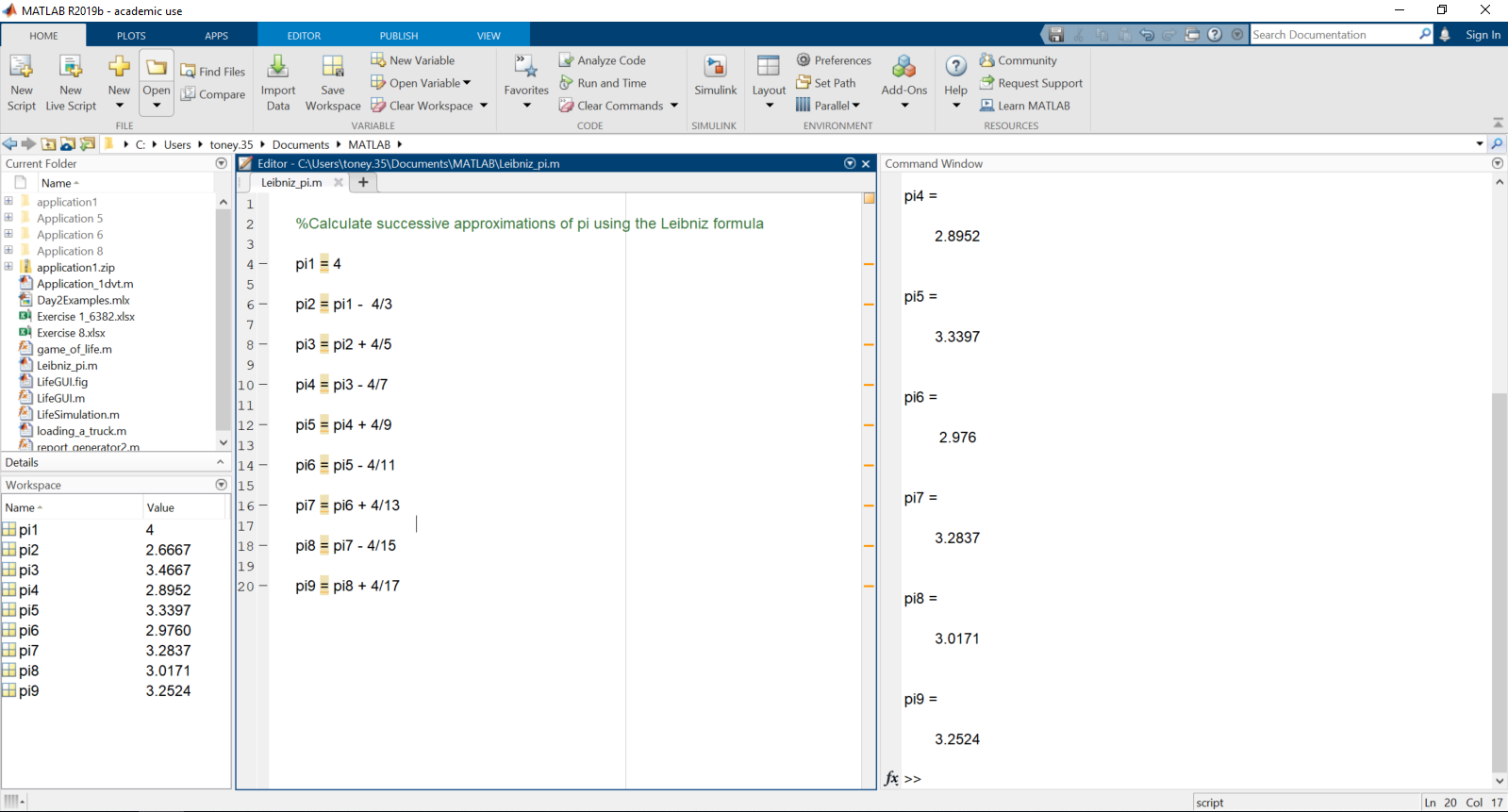
Figure 1.5: A simple script
You can see that this power series is not a very good one – it converges quite slowly.
1.5 Displaying Output
In all of the examples so far, the result of each calculation step was “echoed” to the command window. In most programs that behavior is not desired; it is better to only display the final result. To suppress the output from a calculation step (prevent it from appearing in the command window), terminate the line with a semi-colon. The previous example could be modified so that only the last result is displayed:
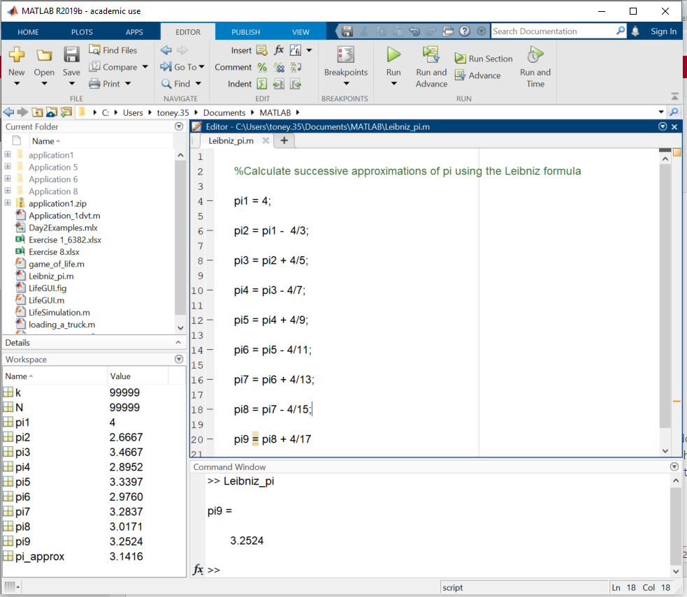
Figure 1.6: Suppressing output using semi-colons
1.5.1 Using disp() to control output
An even better option is to terminate every line with a semi-colon and use the disp() function (or fprintf(), which is introduced in Chapter 3) to control what is displayed to the command window. disp() takes as an argument either a string in quotes (what computer scientists call a ‘literal’) or a variable name. Text in quotes will be displayed exactly as it is; if a variable name is provided, the value of that variable will be displayed. Use of disp() to display the results of the Leibniz_pi script is shown below.
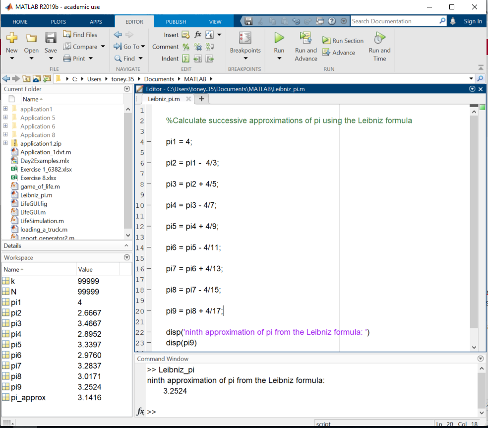
Figure 1.7: Using the disp() function
Improved disp() Functionality
The latest versions of MATLAB allow text and numerical values to be displayed on a single line as follows:
>> disp ("The ninth approximation of pi from the Leibniz formula is " + pi9)
The ninth approximation of pi from the Leibniz formula is 3.2524
>>
The + is a short-cut method for concatenating strings. The number, pi9, is automatically converted to text and appended to the string in quotes.
Important syntax notes: to combine text & numerical output using this method, the text must be enclosed in double-quotes (“) not single-quotes (‘). The reason for this distinction is explained in Chapter 2. Also, the items (text and numbers) are combined using a +, not a comma.
1.5.2 clear and clc
Two commands that are often placed at the beginning of a MATLAB script are clear and clc. It is important to understand the difference between them. clc simply clears the command window – like erasing a white board. clear, on the other hand, erases everything from the workspace – that is, it deletes all of the stored variables from the computer’s memory. It should be used with caution, and never in the middle of a program unless you are sure that you want to throw away all previous results. This is how the previous MATLAB environment appears after executing clear and then clc:
![]()
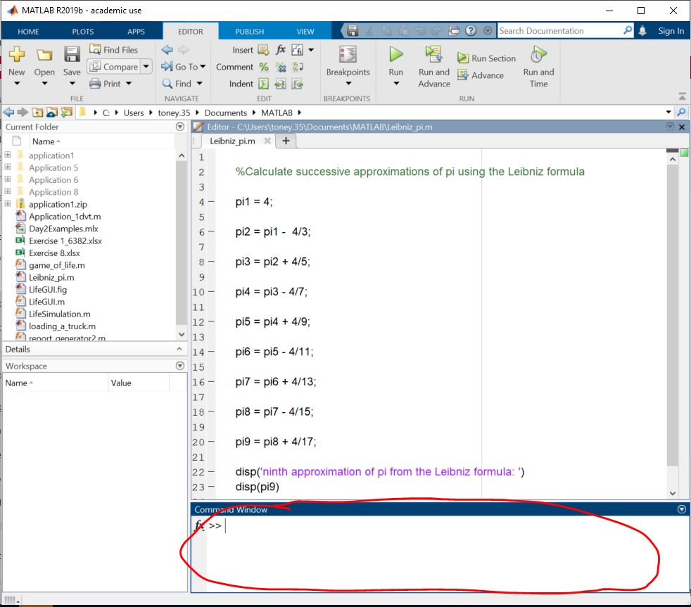
Figure 1.8: The clc and clear commands
For this initial example, it was important to show where in the MATLAB environment the code and output appear using screenshots, but that is not practical for more complex examples. In subsequent chapters, code snippets will be displayed in simple text boxes. Longer code examples with output will be presented as downloadable pdf files like this:
Lecture Video – Scalar Operations
Checkpoint 1.6
1.6 Related Products and Toolboxes
As a proprietary product, MATLAB offers a number of supplemental capabilities beyond the core functionality, which may or may not be included in your license. [2] In this book, we will limit the coverage to core MATLAB, with a few exceptions that will be noted. Some of the most commonly used products and toolboxes are:
- Curve Fitting Toolbox
- Signal Processing Toolbox
- Image Processing Toolbox
- Symbolic Math Toolbox
- Statistics and Machine Learning Toolbox
- Partial Differential Equations Toolbox
- Simulink
The last of these, Simulink, is really a separate product that enables block-diagram-based simulation models of dynamic systems.
Since MATLAB requires a paid license, it may not be accessible to users who do not belong to a university or other large organization. For those users, there are some open-source alternatives to MATLAB that have comparable core functionality:
- Octave
- Scilab
- Python with Numpy and Matplotlib
Of these, Octave is the most nearly MATLAB-compatible. Most MATLAB programs that use only core functionality will run without modification in Octave. Scilab has some differences in syntax, so porting programs between it and MATLAB will require some edits. Python is not similar to MATLAB in syntax, but with the addition of two libraries – Numpy for array operations and Matplotlib for plotting – it has comparable functionality. Porting a program from one to the other would be non-trivial, but a generative AI tool like ChatGPT could probably handle that task easily.
1.7 Mathworks Resources
1.8 Problems
1. Plane stress transformation: Given randomly generated values of [latex]\sigma_x, \sigma_y[/latex], [latex]\tau_{xy}[/latex], and θ, calculate the normal stress ([latex]\sigma_n[/latex]) and shear stress ([latex]\tau_{nt}[/latex]) on an inclined plane from the following equations:
3. The decibel scale is a logarithmic scale that is widely used in electromagnetics and acoustics. In acoustics, the relationship between the sound intensity in [latex]W/cm^2[/latex] and the sound pressure level in decibels (dB) is
4. In radioactive decay, the number of active nuclei decreases with time according to the equation
[latex]N(t) = N_0 e^{-t/\tau}[/latex]
where [latex]\tau[/latex]is the decay time constant. It is related to the half-life by
5. Calculate the following approximations of [latex]\pi[/latex] and the percent error in each. All errors should be much less than 1 %.
6. Trigonometric Identities
Put this line at the beginning of your script:
x = pi*rand()i is a built-in constant, equal to [latex]\sqrt{-1}[/latex]%This is the number of slices per pizzaSLICES_PER_PIZZA = 6;%These are the people who want cheese; the number of slices for each person is generated randomlyRachel_cheese = randi([1,3]); %this generates a random integer between 1 and 3Joey_cheese = randi([3,5]);Ross_cheese = randi([2,4]);%These are the people who want pepperoniPheobe_pepperoni = randi([1,4]);Monica_pepperoni = randi([2,3]);Joey_pepperoni = randi([2,4]);Chandler_pepperoni = randi([2,4]);%Generate random values of a and b for both parts, gamma for part (a) and alpha for part (b)%NOTE: the values of gamma and alpha may not be consistent with each other; don't worry about that - the two parts%of the problem are independenta = 2*rand();gamma = 90*rand();alpha = 90*rand();b = min(rand(), a/sind(alpha)); %Limit b so that there is a real solutionlambda = randi([454, 700])*1.0e-9;10. In Imperial units, the ounce is sometimes used a measure of volume and sometimes as a unit of weight. Calculate the weight in ounces (oz.) of 1.0 fluid ounce (fl. oz.), of water at standard temperature and pressure using the following values:
[latex]\\[/latex]
- The first convention, with underscores, is sometimes called "snake case", while the latter, with capitalization, is called "camel case". ↵
- If you use MATLAB Online, all products and toolboxes that are included in your institution's license will be available. If you are using MATLAB on your local computer, you must select the products and toolboxes that you want to include in your installation. ↵
