12 Graphical User Interfaces

A crucial and often-overlooked aspect of modern software is the user interface. In the first few chapters, interaction between the user and the program was limited to simple command-line input & output. Chapter 11 introduced some simple graphical input & output capabilities – dialog and message boxes. This chapter discusses full graphical user interface (GUI) programming using the App Designer utility. While GUI programming can be complex, App Designer automatically generates the user interface code, allowing the programmer to focus on the computational aspects of the app.

12.1 Graphical Objects and Handles

Before delving into GUI design with App Designer, it is important to understand the concept of a graphical object “handle.” First, a graphical object is a structure that the user interacts with. Examples that we have covered so far include figure windows, plots, axes, dialog boxes and message boxes. Some additional graphical object types that are discussed in this chapter are buttons, menus, and text or numeric entry fields. The handle to a graphical object is a reference to the object that enables a program to interrogate or change the properties of the object.

As a first example of using graphical object handles, consider creating a figure window, axes, and plot, while assigning a handle to each of these objects, so that the properties can be modified later in the program.

>> fig1 = figure();

>> ax1 = axes();

>> pl1 = plot(xvals, yvals);

fig1, ax1, and pl1 are handles that can be used to inspect or change the properties of the objects. “Properties” includes a wide range of attributes, such as size and position on the screen, font size and color, line style and width, etc. The list of properties of an object can be seen two ways:

1. display the object from the command window:

>> fig1

Figure (1) with properties:

Number: 1
Name: ''
Color: [0.9400 0.9400 0.9400]
Position: [360 198 560 420]
Units: 'pixels'

Show all properties

When “all properties” is clicked, the full list is displayed:

Alphamap: [1×64 double]
BeingDeleted: ‘off’
BusyAction: ‘queue’
ButtonDownFcn: ”
Children: [1×1 Axes]
Clipping: ‘on’
CloseRequestFcn: ‘closereq’
Color: [0.9400 0.9400 0.9400]
Colormap: [256×3 double]
CreateFcn: ”
CurrentAxes: [1×1 Axes]
CurrentCharacter: ”
CurrentObject: [0×0 GraphicsPlaceholder]
CurrentPoint: [0 0]
DeleteFcn: ”
DockControls: ‘on’
FileName: ”
GraphicsSmoothing: ‘on’
HandleVisibility: ‘on’
InnerPosition: [360 198 560 420]
IntegerHandle: ‘on’
Interruptible: ‘on’
InvertHardcopy: ‘on’
KeyPressFcn: ”
KeyReleaseFcn: ”
MenuBar: ‘figure’
Name: ”
NextPlot: ‘add’
Number: 1
NumberTitle: ‘on’
OuterPosition: [353 191 574.6667 507.3333]
PaperOrientation: ‘portrait’
PaperPosition: [1.3333 3.3125 5.8333 4.3750]
PaperPositionMode: ‘auto’
PaperSize: [8.5000 11]
PaperType: ‘usletter’
PaperUnits: ‘inches’
Parent: [1×1 Root]
Pointer: ‘arrow’
PointerShapeCData: [16×16 double]
PointerShapeHotSpot: [1 1]
Position: [360 198 560 420]
Renderer: ‘opengl’
RendererMode: ‘auto’
Resize: ‘on’
Scrollable: ‘off’
SelectionType: ‘normal’
SizeChangedFcn: ”
Tag: ”
ToolBar: ‘auto’
Type: ‘figure’
UIContextMenu: [0×0 GraphicsPlaceholder]
Units: ‘pixels’
UserData: []
Visible: ‘on’
WindowButtonDownFcn: ”
WindowButtonMotionFcn: ”
WindowButtonUpFcn: ”
WindowKeyPressFcn: ”
WindowKeyReleaseFcn: ”
WindowScrollWheelFcn: ”
WindowState: ‘normal’
WindowStyle: ‘normal’Units: ‘pixels’

Any of these properties can be changed by an assignment statement. For example, to change the background color of the figure to blue-green:

>> fig1.Color = [0, 0.5, 0.5];  %RBG values

2.) Click on the object in the workspace. This will open the Property Inspector:

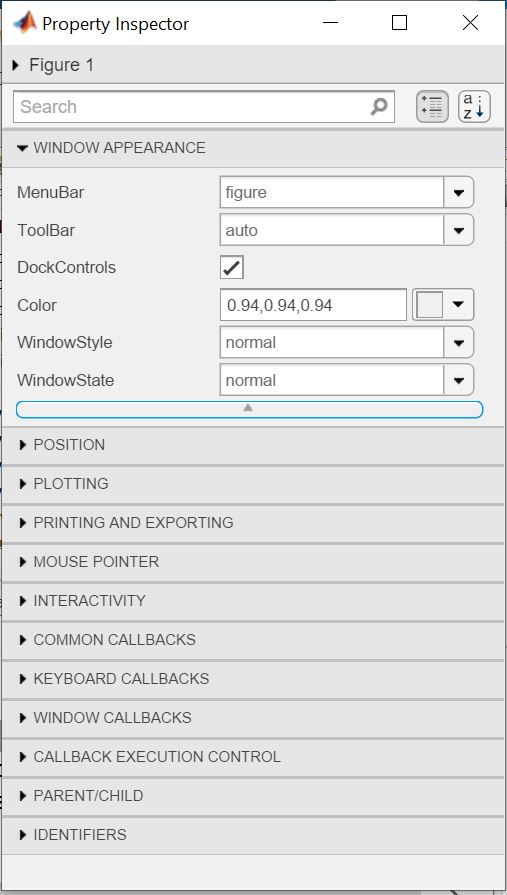
In this window, the properties can be both viewed and changed, by editing the values in the edit fields.

The following example shows how the properties of a plot can be changed under program control. Suppose that the function temperature_measurement() reads a temperature value from a sensor, and the function PID() applies a control signal to a temperature controller. The program continuously makes measurements and plots them. If the temperature exceeds the maximum permitted level, the plot line color is changed to red as a warning.

12.2 Drawing Simple Figures with patch

MATLAB has a simple polygon-drawing function called patch() that is useful for creating basic figures and animations. To illustrate the use of the function, this example will draw a block-O figure by overlaying several polygons. For each polygon, you must provide 3 things:

• a vector with the x-coordinates of the vertices
• a vector with the y-coordinates of the vertices
• a color

First, the outer red octagon:

%make vectors containing the x-coordinates and the y-coordinates

X1 = [0, 3, 4, 4, 3, 0, -1, -1 0];

Y1 = [0, 0, 1, 6, 7, 7, 6, 1, 0];

%provide the coordinate vectors and the color (there are numerous other

%options - see the documentation

patch(X1, Y1, 'red')

%Going to overlay another patch, so turn hold on

hold on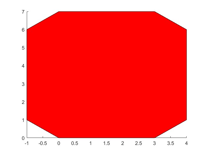

The resulting figure is:

Next, the inner white octagon:

%Repeat for the second patch

X2 = [1, 2, 3, 3, 2, 1, 0, 0 1];

Y2 = [1, 1, 2, 5, 6, 6, 5, 2, 1];

patch(X2, Y2, 'white')

%scale the axis to get the right appearance

axis equal

axis([-2, 5, -1, 8])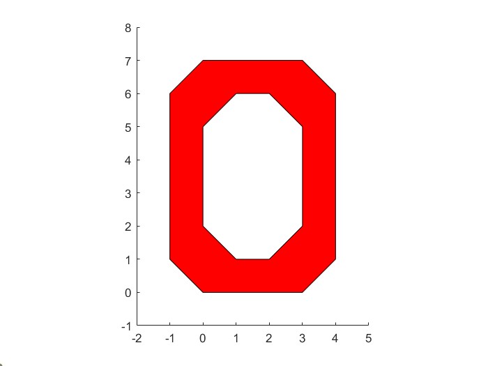

Resulting figure:

Now, the inner black edge:

%Can also make the edges a different color than the face

X3 = [1.25, 1.75, 2.75, 2.75, 1.75, 1.25, 0.25, 0.25 1.25];

Y3 = [1.25, 1.25, 2.25, 4.75, 5.75, 5.75, 4.75, 2.25, 1.25];

patch(X3, Y3, 'white', 'EdgeColor', 'Black', 'LineWidth', 1.5)

 Resulting figure:

The block-O is still not quite complete – the outer black edge is missing. Adding it is left as an exercise.

12.3 GUI Programming with App Designer

Writing a full graphical user interface with menus, buttons, and other graphical objects is a complex undertaking. Fortunately, Mathworks provides a utility, App Designer, that automates much of the process. With App Designer, a GUI can be designed simply by clicking and dragging objects onto a palette,  then making a few edits in the Property Inspector to change the appearance as desired.

Since it is difficult (and tedious) to describe an interactive program in text, watch this video for an introduction to App Designer. The simple app described here shows 3 of the most basic operations in an app:

• reading values from an edit field (user-entered parameters)
• responding to a button press
• displaying results to a text label

Another method of user input in an interactive program is mouse clicking. This video demonstrates an app that detects where on a figure a mouse click occurred and takes a different action depending on the clicked coordinates.

A widely used feature in interactive programs is a drop-down menu. This video demonstrates how to add a menu to an app and how to determine which menu item was selected by the user.

In a GUI program, which is highly modular, sharing of information among callback functions is a key issue. This video shows how to use global variables for that purpose. (A more modern technique is the use of app properties, which is not covered here. See this Mathworks page for more information: https://www.mathworks.com/help/matlab/creating_guis/share-data-across-callbacks-in-app-designer.html)

In some applications, it is desirable to change the appearance of the interface depending on user actions. This video shows one example of a dynamic interface: controlling the visibility of an object.

This video shows how to use a data table, which facilitates user entry or program display of an array of values.

This video demonstrates three GUI features:

• controlling the color and brightness of a lamp indicator
• changing the position of an object under program control
• responding to key presses and performing different actions depending on which key was pressed

12.4 Mathworks Resources

Develop Apps Using App Designer

Graphics Objects

patch – Create patches of colored polygons

12.5 Problems

1. In earlier chapters, you wrote a program to plot a conic section, given the input coefficients A, B, C, D, E, and F. In thisproblem, you will write a graphical user interface for that program in App Designer.

   The GUI should have the following elements:

   • A static text label with a title for the app
   • An input panel with 6 numeric edit fields for the coefficients. To the right of each edit field should be a text label indicating which term of the equation. For example, to the right of the A edit field should be a label reading “x^2”
   • A set of axes to plot the curve
   • A Plot button; the curve is plotted when the button is pressed
   • A text label indicating the type of curve (Parabola, Ellipse, Circle, or Hyperbola; could also include Line if you completed that optional part of Application 3). It is not necessary to display the equation, since it can be read from the input fields.
   • A Reset button. When the button is clicked, all input fields should be set to their default values, the axes should be cleared, and the output text label should be set to an empty string

   Note: For the plotting commands, it is necessary to specify the axes in the GUI so that the plot will be done in the app, not in a separate figure window. See the MATLAB documentation for the plot, xline, xlim, and axis functions for guidance on how to do that. 

    

2. Use the patch function to draw your university’s (or alma mater’s or favorite sports team’s) logo.

   3. In this assignment you will write a MATLAB app to simulate a common introductory physics experiment – aiming a launched projectile so that it lands in a box. The position of the launcher and the box are fixed, and the projectile is aimed by adjusting the launch angle, as shown in the figure. ^[1] 

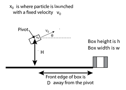
    The projectile is treated as a point particle, and air resistance is neglected. The trajectory of the particle can be calculated from basic kinematics as

[latex]y = H +\frac{l}{2}\sin \theta + \tan \theta (x-\frac{l}{2} \cos \theta) - \frac{1}{2} g (\frac{x-\frac{l}{2} \cos \theta}{v_0 \cos \theta})^2[/latex]

where

H = height of table

l = length of launcher

v₀ = initial speed of projectile

[latex]\theta[/latex] = launch angle relative to the horizontal

g = acceleration of gravity = 9.81 m/s²

Additional parameters:

D = distance from edge of table (x=0) to front edge of box

h = height of box

w = width of box

• • Create a MATLAB app with a GUI that allows the user to enter H, l, v0, D, h, w, and theta as parameters. All edit fields should have valid values on startup and reasonable limits should be set (for example, all values must be positive).
  • The input fields should be grouped into a panel
  • Calculate the trajectory and plot y vs. x in the GUI axes (not a separate figure). Only plot the trajectory until the projectile hits the floor (y>=0).
  • On the same figure, use the patch command to draw the box. If the particle enters the box through the top opening, draw the box in green; if it misses, draw the box in red.
  • Display a message to a text label that indicates Hit or Miss.

Choose one of the following input methods:

• • Enter theta in an edit field, and include a calculate button; run the calculation and plot the results when the button is clicked
  • Use a slider to adjust theta; update the calculations and graph whenever the slider position is changed.

In either case, set the limits on theta to be [0, 90].

Print a text message (label) to the GUI telling the user whether the projectile hit or missed.