4 Logical Arrays and Data Analysis

For a computer program to have “intelligence”, it must be able to make decisions. The way computers do that is by making comparisons, such as “Is this variable greater than that one?” or “Is this variable equal to a certain value?” The operators that perform these comparisons are called relational operators. In many cases, it is useful to evaluate two or more conditions simultaneously; boolean operators (and, or and not) are used in conjunction with relationals to evaluate more complex conditions.

This chapter introduces the concepts of relational and boolean operations and shows how they are applied to arrays. Chapter 6 discusses use of relational and boolean expressions with the if statement to make decisions (branching) in a program.

4.1 Relational Operators and Logical Values

Decision-making in computer programs is typically driven by logical comparisons: one action is performed if a condition is true, while another is performed if it is false. Conditions are expressed in terms of a comparison of two quantities by applying one or more of the following relational operators:

>         greater than
<         less than
>=       greater than or equal to
<=       less than or equal to
==       is equal
~=       is not equal

The result of applying one of these operators is either true (logical 1) or false (logical 0).

A few basic examples are shown below:

>> x = 5;

>> x > 4

ans =

logical

1

>> x < 4

ans =

logical

0

>> x == 15/3

ans =

logical

1

The result of relational operations can be stored in a variable for later reference:

>> x_is_negative = x<0

x_is_negative =

logical

0

It is a bad practice to apply the equality operator (==) to expressions involving floating-point numbers. Because of the finite precision with which numbers are stored in a computer, roundoff error will often cause values that should be equal to be unequal. For example:

>> lhs = 1 + (1/3) - 2*4.0/8.0

lhs =

0.3333

>> rhs = 1/3

rhs =

0.3333

>> lhs == rhs

ans =

logical

0

Although these two expressions are mathematically equal, their digital representations are slightly different. This can be seen by calculating the difference:

>> lhs - rhs

ans =

-5.551115123125783e-17

The usual practice with floating-point numbers is to set a tolerance and regard any value less than that tolerance as zero:

>> tolerance = 1.0e-9;
>> abs(lhs - rhs) < tolerance

ans =

logical

1

4.2 Boolean Operators

In some cases, a decision is based on multiple conditions being true simultaneously. In other cases, it may be based on one of several conditions being true. It is common to make decisions this way in everyday life, as in these examples:

• I will go to see Top Gun: Maverick tomorrow if it is showing in the IMAX theater AND there are tickets available for the 7:00 show.
• I will take that job if they give me a raise over my current salary OR they give me a bigger office.
• I will go cycling this afternoon if it does NOT rain

In the first example, both conditions have to be true for the decision to be taken. In the second, if either or both conditions are true, the decision is taken.

In MATLAB and other programming languages, these kinds of compound conditions are implemented using boolean operators. These operators return a true (logical 1) or false (logical 0) result, depending on the values of the operands, as summarized in Table 4.1.

Table 4.1 : Boolean Operators

Boolean operators are commonly used in conjunction with relational operators, as in this example:

    >> x_is_real_positive = imag(x) == 0 && x > 0

This expression evaluates to true (logical 1) if and only if both conditions are true: x is real (its imaginary part is 0) and x is positive (greater than 0).

    >> x_is_real_positive = imag(x) == 0 && x > 0

Another example, using the or operator:

    >>     y_outside_limits = y < 10 || y > 20

This expression is true if y is NOT between 10 and 20 inclusive.

See MATLAB help page

4.3 Order of Operations & Mixed Arithmetic-Logical Expressions

Relational and boolean operators can be combined with arithmetic operators to achieve something much like branching with an if statement (see Chapter 6). The key to using this technique is to understand two things:

1. In MATLAB, boolean operators treat any number other than 0 as true, as in these examples:

>> ~100

ans =

logical

0

>> x = 3;
>> y = -1;
>> x && y

ans =

logical

1

>> y || 0

ans =

logical

1

   2. When a logical 0 or 1 appears in an arithmetic expression, it is treated as an arithmetic 0 or 1, as in these examples:

>> w = x == 3

w =

logical

1

>> z = y < 0

z =

logical

1

>> w + z

ans =

2

Relational expressions can be added, and the result is the number of the expressions that are true. For example,

>> (pi > 3) + (exp(1) < 3) + (sin(pi/4) == cos(pi/4))

ans =

2

The first two of these expressions are unambiguously true; the third is true mathematically, but evaluates to false in a computer due to the finite precision with which floating-point numbers are represented. (Review section 4.1.)

This technique can be used to accomplish something much like and if…else structure, which is discussed in Chapter 6.  Suppose you want to accomplish this operation:

• if x is positive, let y = 10
• if x is 0 or negative, let y = 20

One way to accomplish that is with this expression:

y = 10*(x > 0) + 20 * (x <= 0)

Since the two relational operators are complementary (assuming that x is real),  one of the two terms is true (1), and the other is false (0); thus y will have the value 10 or 20, as intended:

>> x =-3;

>> y = 10*(x > 0) + 20 * (x <= 0)

y =

20

When arithmetic, relational, and boolean operators are combined in a complicated expression, the order of operations is as shown in this table:

With the exception of the not (~) operator, which is relatively high in precedence, the general order is arithmetic > relational > boolean.

See MATLAB help page

4.4 Logical Arrays

When a relational operator is applied to an array, the result is a logical array – an array of true/false values (also called logical 1 / logical 0). For example, if these commands are executed:

>> A = 0:2:10;

>> A_gt_4 = A > 4  %Are the elements of A greater than 4?

A_gt_4 =

1×6 logical array

0 0 0 1 1 1

The first 3 elements of the resulting logical array are logical 0 (false), since the first 3 elements of A are not greater than 4. The last 3 elements are logical 1 (true), since the corresponding elements of A are greater than 4.

Multiple relational operators can be combined with boolean operators to determine which elements of an array meet a complex condition. For example, to determine which elements of A are between 5 and 9, inclusive:

>> A_bt_5n9 = A >= 5 & A <= 9

4.5 Logical Indexing and the find() Function

A powerful technique for analyzing data arrays is to use a logical array as an index; this picks out the values of the data array for which the logical array is true. This technique, logical indexing, is typically used in conjunction with a relational operator to choose the elements of an array that meet a certain condition. For example, suppose you want to take the average of only the positive numbers in an array:

>> X = [-5, 7, -2, -4, 8, 3, 0, -6, 5];

X_pos = X (X > 0)

X_pos =

7 8 3 5

>> avg_pos = mean (X_pos)

avg_pos =

5.7500

>>

The expression X (X > 0) picks out only those elements of X that meet the condition, X > 0.

Logical indexing can also be used between two arrays, provided that they have the same dimensions. Suppose there are two arrays containing daily high temperatures and precipitation levels. To pick out the high temperatures on the days when it rained or snowed:

>> temperature = [41, 37, 28, 23, 36, 44, 50];

>> precipitation = [0, 0, 1.2, 0.3, 0, 2.5, 0.3];

>> temp_wet_days = temperature (precipitation > 0)

temp_wet_days =

28 23 44 50

Logical indexing is used to extract the values of an array that meet a certain condition. In some cases, it is useful to know the indices of the elements that meet the condition. For example, in the previous example, we may want to determine the days when the high temperature was below freezing. The find() function is useful for this type of analysis. Fundamentally, find() returns the indices of all non-zero elements in an array. It is often used in conjunction with a logical array to find the indices of the elements that satisfy a condition.

>> freezing_days = find(temperature < 32)

freezing_days =

3 4

This tells us that the 3rd and 4th days had sub-freezing high temperatures.

The find() function can also return the index of the first or last occurrence(s) of a condition. For example, to determine the last day when the temperature was below freezing:

>>last_freeze = find (temperature < 32, 1, 'last')

last_freeze =

4

Replace 'last' with 'first' to determine the first occurrence of the condition. The number 1 can be replaced by any positive integer, n, to determine the first or last n occurrences.

4.6 Mathworks Resources

Relational Operations

Logical (Boolean) Operations

4.7 Problems

1. Download this data file and move it to your MATLAB folder. The file contains a 2D array with daily average global temperature anomaly from 1880 through 2018. The data are organized as follows:

2. For the data set of the previous problem, on 3×1 subplot, plot the temperature anomaly vs. time for three periods: 1880 – 1925, 1926-1971, and 1972 – 2017. For the horizontal axis data, use: year + month/12 + day/365. Make the vertical and horizontal scales of each plot the same, so that the trends can be compared visually. Make sure that the plot is fully annotated.

[latex]\\[/latex]

3. The Goldbach conjecture  states that every even whole number greater than 2 is the sum of two prime numbers.  It has never been proven but has been verified for every even number up to [latex]4\times 10^{18}[/latex]. There may be multiple pairs of prime numbers that sum to a given number. For example, 20 can be written as the sum of two primes two ways:  

20 = 3 + 17

20 = 7 + 13

[latex]\\[/latex]

Problem statement: Given an even number, N, entered by the user, find all pairs of primes that sum to N and store them in a matrix called prime_pairs, with each row being one prime pair.

[latex]\\[/latex]

For example, if N = 20, the matrix would be:

prime_pairs = [3, 17; 7, 13]

You can use the built-in function isprime() to determine which numbers are prime. [isprime (n) returns 1 (true) if n is prime, 0 (false) otherwise.]

A suggested approach to this problem is:

i. Create a vector X (or any other name that you prefer), containing the integers 2, 3, 4, … N/2 (It’s not necessary to go all the way to N, since that would double-count the prime pairs)

ii. Create a second vector, Y (or any other name that you prefer), equal to N – x

iii. Create a logical array that is true if and only if both X and Y are true (use the isprime function and a boolean operator)

iv. Using logical indexing with the logical array from part 3, pick out only those values from X and Y that belong to the prime pairs. (You can either create two new vectors or modify the X & Y vectors.)

v. Concatenate the vectors created in part 4 side-by-side to create the matrix prime_pairs.

As a test case, run your program with N = 98. The resulting prime pairs should be [19, 79; 31, 67; 37, 61]

[latex]\\[/latex]

4. Monte Carlo Integration of a Volume

In this problem, you will compute the (approximate) volume of an ellipsoid by a Monte Carlo method. This method involves generating a large number of (x, y, z) coordinates at random, and counting the number that lie within the solid. The fraction of points that fall within the solid is equal to the ratio of the volume of that solid to the volume of a rectangular prism with the same outer dimensions.

Given:

• • a, b, and c, the lengths of the 3 semi-axes of the ellipsoid
  • N, the number of points in space to generate

Generate three 1xN row vectors of random numbers, X, Y, and Z, using the rand()function. Since rand() returns values between 0 and 1, multiply the 3 random vectors by a,b, and c respectively.

Count the number of points that lie within the ellipsoid using the sum() function with a relational operator. The condition for a point to be inside the ellipsoid is:

[latex]\frac{x^2}{a^2}+\frac{y^2}{b^2}+\frac{z^2}{c^2}<1[/latex]

Since x, y, and z are positive values, only one octant is being counted. Therefore the volume of the total ellipse is:

[latex]V_{approximate} = 8\times\frac{number\ of\ points\ inside\ ellipsoid}{N}\times a \times b \times c[/latex]

The exact volume of an ellipsoid is

[latex]V_{exact} = \frac{4}{3}\pi\ a\ b\ c[/latex]

For some set of positive numbers, a, b, and c, calculate the percent error between the approximate and exact values with N=100000. If it is more than +/- 1 %, you have probably made an error in your calculation.

Repeat the calculation for the same values of a, b, and c with N = 10000, 1000, and 100. Does the approximation become less accurate as N decreases?

[latex]\\[/latex]

5. Character Counting

Copy this line in your MATLAB script to create a character array called declaration:

[latex]\\[/latex]

declaration = 'We hold these truths to be self-evident, that all men are created equal, that they are endowed, by their Creator, with certain unalienable Rights, that among these are Life, Liberty, and the pursuit of Happiness. That to secure these rights, Governments are instituted among Men, deriving their just powers from the consent of the governed, That whenever any Form of Government becomes destructive of these ends, it is the Right of the People to alter or abolish it, and to institute new Government, laying its foundation on such principles, and organizing its powers in such form, as to them shall seem most likely to effect their Safety and Happiness. Prudence, indeed, will dictate that Governments long established should not be changed for light and transient causes; and accordingly all experience hath shewn, that mankind are more disposed to suffer, while evils are sufferable, than to right themselves by abolishing the forms to which they are accustomed. But when a long train of abuses and usurpations, pursuing invariably the same Object, evinces a design to reduce them under absolute Despotism, it is their right, it is their duty, to throw off such Government, and to provide new Guards for their future security.'

[latex]\\[/latex]

a) Count the number of words by counting the blank characters using the sum() function and a relational operator. Store the result in a variable called num_words. The correct answer is 201. (Remember that the number of words is one more than the number of blanks!)

b) Delete all of the commas from declaration. You should be able to do this with a single assignment statement and logical indexing. (You can use the length() function to compare the length of the character array before and after deleting the commas. The difference should be 20.)

[latex]\\[/latex]

6.  Eliminating Non-real Data from a Plot

After completing Problem 2 in Chapter 3 (Plotting Conic Sections), modify your code so that the extraneous lines outside of the conic section are removed. To achieve this, use logical indexing to delete the parts of the data for which y1 and y2 are not real. You can use the imag() function for this purpose. (i.e. delete the x and y values for which the imaginary part of y1 is not equal to zero.)  

Note 1: y1 and y2 will both be real, or they will both be complex, so you don’t have to check both. 

Note 2: There will be a small gap in the graph where the two branches meet; it is not necessary to do anything to eliminate it. You can reduce the gap by using a smaller step size.

[latex]\\[/latex]

7. Logical Expressions and Switching Circuits

Write the logical expressions, using boolean operators, to determine if bulbs A and B are on or off for the following circuit using the variables SW1, SW2, SW3, where closed is true and open is false.^[1]

Use this code to generate three vectors representing all possible combinationsof SW1, SW2, and SW3:

[latex]\\[/latex]

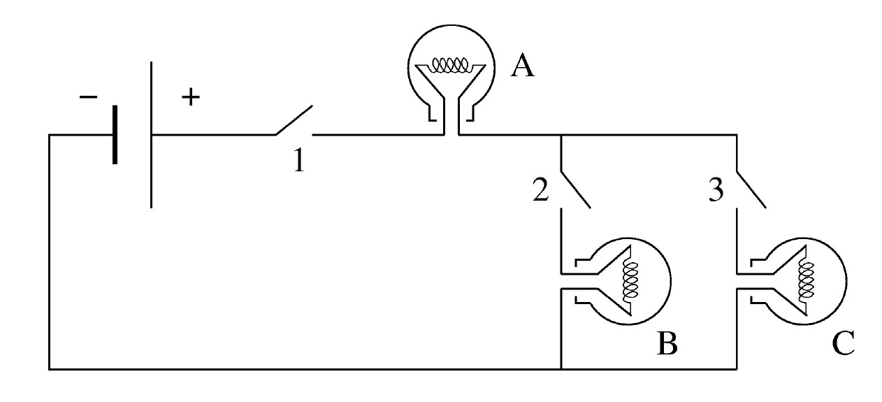
SW1 = [1, 0, 1, 0, 1, 0, 1, 0];

SW2 = [1, 1, 0, 0, 1, 1, 0, 0];

SW3 = [1, 1, 1, 1, 0, 0, 0, 0];

[latex]\\[/latex]

STORE THE RESULTS IN TWO VECTORS CALLED A_on AND B_on. For example, if you think that bulb A will be on if and only if all 3 switches are closed, the expression would be

[latex]\\[/latex]

A_on = SW1 & SW2 & SW3 %not correct

[latex]\\[/latex]

If your expressions are correct, A_on should contain three 1s and five 0s, while B_on should contain two 1s and six 0s.

   8. Upper and Lower-case Characters

Starting with the character array, declaration, from problem 5:

a. Convert the character array into a numerical array of ASCII values by multiplying it by 1 or by using the double() function.

b. Determine how many capital letters are in the text. (The ASCII codes for capital letters are between 65 and 90, inclusive.)

c. Convert the capital letters to lowercase by adding 32 to their ASCII codes. (But do not modify the lowercase letters. Do not use the lower() function.) 

d. Convert the modified array back to text using the char() function and print it to the command window.

Find an error? Have a suggestion for improvement? Please submit this survey.