8 Program Structure

In Chapter 5, when user-defined functions were introduced, a particular scheme was emphasized: each function was stored in a separate file, and all files constituting a given program were stored in a single folder. That is the simplest way to organize a modular program and the best way for novice MATLAB users, but not the only way. This chapter discusses other approaches to organizing a complex program.

8.1 Local Functions

Contrary to the approach taken earlier, a single file can contain multiple functions, but there are restrictions on how those functions can be used.

• Rule #1: Only the first unit of code in a file (either a function or a script) can be called or executed from outside that file; all subsequent functions are local functions – they can only be called from within the same file.
• Rule #2: Even though two or more functions reside in a single file, they have separate workspaces; that is, variables that are defined inside a function only exist while that function is running, and they cannot be accessed by other functions. (The exception, global variables, is discussed later in this chapter.)
• Rule #3: If a program is organized as a main script with local functions in the same file, the script must appear first in the file, followed by the function definitions.
  • Corollary: if there is even a single line of code in a file before a function definition, that line of code is the main script, and the function is a local function. So never put any code (especially a clear statement!) before the function definition line of a stand-alone (external) function.

The following example illustrates the use of a local function. The “main” function ^[1] converts a Roman number in the form of a character array to its decimal equivalent. ^[2] There is a local function, sometimes called a “helper” function, called digit_val(), to perform the sub-task of determining the value of a single Roman digit. The helper function is called by the main function, but it cannot be called externally, as shown in the command window below. Notice that an error occurs when the local function, digit_val(), is called from the command window.

8.1.1 Variable Scope

Rule #2 above is often a pitfall for novice programmers; it is the main reason why it is better to avoid local functions until you gain a fair amount of experience. The following example illustrates the idea of the scope of a variable. A key point is that even though two functions may each have a variable of the same name, they are different variables. The video below explains this example in detail.

8.2 Organization of a Complex Program

The presentation below illustrates how the pieces of a modular program fit together. MATLAB allows tremendous flexibility in constructing a program using local and external functions. With that flexibility comes complexity, but it has the great benefit of allowing easy code re-use. Once a function has been written to accomplish a given task, it can be used in any number of programs.

This presentation leaves open one important question: should the “main” program be a function or a script? Either choice is perfectly valid, provided that you understand the limitations of each approach. The most important differences between a function and a script are:

1. A function can accept input arguments and return output arguments
2. A script preserves the contents of the workspace (unless it contains a clear command), while a function does not

To summarize: if you want to pass arguments to your program, make it a function; if you want the contents of the workspace to be preserved after execution of the program, make it a script.

8.2.1 The Search Path

We have seen that a user-defined function can be local (in the same file as the script or function that calls it) or external (in a separate file). This raises an important question: if there are two functions with the same name, one local and one external, which one will be executed? MATLAB has a sequence, or search path, that it explores when searching for a function definition matching a call. The order of precedence is as follows:

1. local function in the same file as the caller
2. external user-defined function in the same folder as the caller
3. external user-defined function in another folder in the path
4. MATLAB built-in function

Point 3 requires some explanation. To see the list of folders in the search path, execute the path command from the command line. You will see a list something like this:

The list of folders may be long, depending on how many toolboxes are included in your MATLAB license, but it will typically have the top-level MATLAB folder first in the list. A folder can be added to the top of the path using the addpath command:

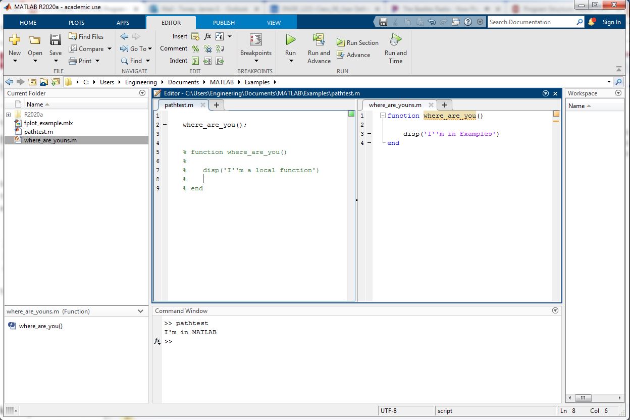
The following sequence of examples illustrates these rules. Note that there is a local function called where_are_you() as well as an external function of the same name in the same folder (Examples) as the script. There is a third version of the function (not shown in the figure) in the MATLAB folder.

Case 1: local function is executed

Case 2: local function is commented out, so external function in the same folder is executed

Case 3: name of external function file in the Examples folder does not match the function call, so the function in the MATLAB folder is executed:

An important point about this last case: notice that the filename and the function name do not match – according to the function definition line it is where_are_you(), but the filename is where_are_youns.m. In that case, the filename takes precedence; so MATLAB regards this function as being called where_are_youns(), regardless of the name in the function definition line.

8.3 Anonymous Functions

In some applications it is useful to have a function to evaluate a mathematical or logical expression. In cases like this, which can be implemented with a single line of MATLAB code, the full structure of a user-defined function is unnecessary. Any function that can be implemented in one line of code can be realized with an in-line or “anonymous” function. An example of defining and using an anonymous function is given below:

The required elements of the anonymous function definition are:

1. function name (rsd in this example)
2. = sign
3. argument list in parentheses [(X) in this example]
4. single line of MATLAB code

Key points about anonymous functions:

1. Unlike local functions, anonymous functions must be defined before they are called.
2. Anything that can be done in a single line of MATLAB code can be implemented as an anonymous function; it does not have to be a mathematical expression. See the next checkpoint question for a slightly challenging example.
3. In most cases, element-wise operations (such as the ./ used in the example) should be used to give the function maximum flexibility to handle array arguments. (In the example, if X is a matrix, the function will return a vector calculated by performing the operation on a column-by-column basis.)
4. An anonymous function can take multiple arguments. That is illustrated by the next example, which expands the previous one by adding a second argument to specify calculation by rows, by columns, or for an entire matrix

8.3.1 Plotting Functions with fplot()

The built-in function fplot() is a convenient way to plot a mathematical function without the need to calculate the values of the independent and dependent variables in advance. It is only necessary to provide a “handle” to the function and the upper and lower limits on the independent variable, and MATLAB handles the rest. The function handle is the name of the function, preceded by the @ symbol; however, if the function was defined as an anonymous function, the @ is not necessary.^[3]

Here is an example of using fplot with a local or external function and with an anonymous function.

With fplot() there is no need to specify a step size; MATLAB will choose an appropriate step size based on the characteristics of the function.

8.4 More on Input & Output Arguments

Chapter 4 stated that a user-defined function has a number of input arguments and a number of output arguments. In special cases, one or both of those numbers can be zero – that is, a function does not strictly require either input or output arguments.

An obvious example of a built-in function that has no output arguments is disp().  To define a function with no output arguments, simply omit the output argument list and = sign, as in this example:

An example of a built-in function that has no input arguments is clock, the function that returns the current time as an array in the form [year month day hour minute second]. To define a function with no input arguments, simply leave the parentheses empty, as in this example:

8.4.1 Variable Number of Input Arguments

It is often useful for a function to perform different operations depending on how it is called. We saw this previously with many of the built-in functions, as in these two calls to the min() function:

User-defined functions can also accept a variable number of input arguments. The built-in variable, nargin, can be examined to determine how many arguments were passed to the function when it was called, and the function can take different actions as appropriate.

The following example illustrates use of nargin to implement an arctangent function that supersedes four separate built-in functions: atan(), atan2(), atand(), atan2d(). atan() takes a single argument, which means that it cannot distinguish between angles in the 1st and 3rd (or 2nd and 4th) quadrants. atan2() takes two input arguments, a numerator and denominator, so it preserves quadrant information. atand() and atan2d() are similar, but return the angle in degrees instead of radians.

The function shown in this example can take a single argument, in which case it calls atan(); two arguments, in which case it calls atan2(); or three arguments, the third one being a unit specification, in which case it calls atand() or atan2d().

This example uses a few interesting techniques. Notice:

• under case 2, the use of isnumeric() to determine if the second argument is a number (in which case, atan2() is called) or text (in which case it represents units).
• under case 2, in the else clause, the use of recursion – that is, the function calling itself. This is a shortcut that helps to keep the logic less messy. Once it is determined that the second argument is a units string, the arctan() function is called again with a denominator of 1, which produces the same result as calling atan() or atand().
• under case 3, the use of lower() to make sure that the units string (actually, a character array) is lower-case, again to simplify the logic. By only looking at the first character, the function allows the units to be expressed in various ways, e.g. ‘degrees’, ‘Deg’, ‘D’, etc.

8.5 Global Variables

One of the most important points in this chapter is that each function has its own set of variables that cannot be accessed by other functions (Rule #2). However, there are times when it is convenient to allow multiple functions to share variables, to avoid having to pass a lot of information through argument lists. This is especially useful in Graphical User Interface programming.

For a variable to be shared between functions (or a main script and a function) it must be declared as global. The following example shows how a script and a function can share a global variable. Notice that func1 does not have a global x declaration; therefore it uses its own variable x, which gets its value from the caller through an input argument. In func2, on the other hand, the input argument is z, and the value of x comes from the global variable. Notice that after performing its calculation, func2 changes the value of x; since the script shares the same global variable, the value of x has changed in the script as well.

8.6 Mathworks Resources

For more details about functions and program structure, see these Mathworks web pages:

Functions

Find an error? Have a suggestion for improvement? Please submit this survey.