10 Reading & Writing Files
MATLAB is commonly used for analysis of large data sets, which are typically read from a file. The file may have been generated by a data acquisition system or downloaded from a web page. Most often it is in ASCII (plain text) or spreadsheet (e.g. Excel) format.
MATLAB contains numerous built-in functions for reading and writing files of various formats. Some of those functions, like xlsread and xlswrite are “deprecated” – meaning that they still exist, but their use is no longer recommended. (If you use a deprecated function, MATLAB may give you a warning and recommend a different function.) It is best to avoid using deprecated functions, since they may be removed from future MATLAB releases.
This chapter presents a few of the most common methods for reading and writing numerical and text data from/to files.
10.1 Saving & Loading Variables
10.1.1 The .mat (workspace) file
The simplest way to store results from a MATLAB program is to write the value of one or more variables to a file using the save command. Executing save with no arguments saves the contents of the entire workspace to a file called matlab.mat. This is a binary file format that can only be read by MATLAB. This is a quick and easy way to save the current state of the workspace so that it can be restored later and avoid having to repeat calculations.
A .mat file can be loaded back into the workspace with the load command. If load is executed without arguments, MATLAB assumes that the file name is matlab.mat and that it is a binary file. The example below shows loading, clearing and restoring the workspace. In the first frame (upper left), a number of variables are listed in the workspace. In the second frame (upper right), the save command is executed, and the matlab.mat file appears in the current directory. In the third frame (lower left), the clear command is executed, emptying the workspace. In the fourth frame (lower right), the load command is executed, restoring the variables with their previous values to the workspace.
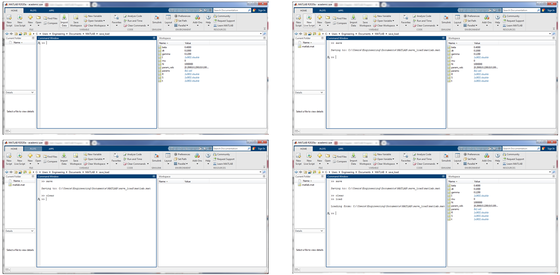
Figure 10.1: Loading and saving variables from the workspace
The workspace can also be saved under a different file name by giving the name after the save command, or in parentheses and quotes after save [1]:
>> %These two commands do the same thing
>> save application10.mat
>> save ('application10.mat')
Similar syntax can be used to load a file with other than the default file name:
>> %These two commands do the same thing
>> load application10.mat
>> load ('application10.mat')
In some cases, you only want to store or load selected variables rather than the entire workspace. In that case, the function form of save() is used, with the variables to be saved given by name (in quotes) after the filename. This command saves the values of the array param_vals to a file called app10_params.mat:
>> save('app10_params.mat', 'param_vals')
Similarly, a specified list of variables can be loaded from a .mat file:
>> %only loads the array param-vals; ignores the rest of the file contents
>> load('matlab.mat', 'param_vals')
10.1.2 Saving, Typing, and Loading ASCII Files
Saving and restoring a MATLAB binary file is appropriate for storing the current state of a session for resumption later, or for sending results to another MATLAB user. More commonly, results are exported from MATLAB for importation into another piece of software, such as Excel or Labview. To save a variable in ASCII (standard text) format, use the functional form of save() with the '-ASCII' switch:
>> save ('app10_params.txt', 'param_vals', '-ASCII')
To examine the contents of a text file from the MATLAB command line, the type command can be used:
>> type app10_params.txt
2.0000000e-01
1.2000000e-01
0.0000000e+00
1.0000000e-01
1.0000000e+06
1.0000000e+02
3.6500000e+02
Notice that the text file created by save() contains only the numbers, not the variable name, and that the numbers are stored in the default format – scientific notation with 7 decimal places. The next section will show how to save numbers to a text file while controlling the format.
The load command can be used to load values from an ASCII file, provided that it has a regular format. Specifically, the file must have the same number of columns in each row. The values will be stored in a single array, the name of which can be specified when calling the load function:
>> paramVals = load('app10_params.txt')
paramVals =
0.2
0.12
0
0.1
1e+06
100
365
If no variable name is specified, it will be the same as the file name minus the extension (in this example, app10_params).
WARNING: bad results can follow from mixing up the syntax for loading a .mat file with that for loading an ASCII file. When loading a .mat file, do NOT use variable_name = load(...). This will cause the variables that were stored in the .mat file to be loaded into a special data structure called a struct, which will be introduced in the next chapter:
>> save application10.mat>> clear>> X = load('application10.mat') %You generally DON'T want to do this!X = struct with fields: I: [1×3651 double] N: 1000000 R: [1×3651 double] S: [1×3651 double] beta: 0.4000 dt: 0.1000 gamma: 0.1200 mu: 0 param_vals: [8×1 double] params: {8×1 cell} t: [1×3651 double]Lecture Video 10.1 – Load and Save
Checkpoint
10.2 Reading and Writing Regular Numerical Data with readmatrix(), writematrix()
To import numerical data from a spreadsheet file, the readmatrix() function should be used. [2] This function is most appropriate when the spreadsheet file has a regular, column-oriented structure. Any non-numerical or empty cells are read as NaN (not a number).
Consider the spreadsheet file shown here:
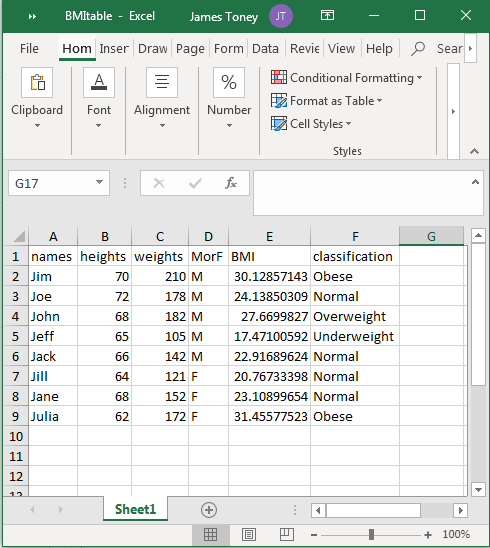
The result of reading this file with readmatrix() is as follows:
>> BMImatrix = readmatrix('BMItable.xlsx')
BMImatrix =
NaN 70.0000 210.0000 NaN 30.1286 NaN
NaN 72.0000 178.0000 NaN 24.1385 NaN
NaN 68.0000 182.0000 NaN 27.6700 NaN
NaN 65.0000 105.0000 NaN 17.4710 NaN
NaN 66.0000 142.0000 NaN 22.9169 NaN
NaN 64.0000 121.0000 NaN 20.7673 NaN
NaN 68.0000 152.0000 NaN 23.1090 NaN
NaN 62.0000 172.0000 NaN 31.4558 NaN
Note that the non-numerical values have been replaced by NaNs. To avoid this occurrence, a range specifier can be used to read only the numerical columns. For example, to read columns B through C:
>> BMImatrix = readmatrix('BMItable.xlsx','Range', 'B:C')
BMImatrix =
70 210
72 178
68 182
65 105
66 142
64 121
68 152
62 172
Unfortunately the range must be continuous, but column E can be read separately and appended to the matrix as follows:
>> BMImatrix = [BMImatrix, readmatrix('BMItable.xlsx','Range', 'E:E')]
BMImatrix =
70.0000 210.0000 30.1286
72.0000 178.0000 24.1385
68.0000 182.0000 27.6700
65.0000 105.0000 17.4710
66.0000 142.0000 22.9169
64.0000 121.0000 20.7673
68.0000 152.0000 23.1090
62.0000 172.0000 31.4558
If the spreadsheet file contains multiple worksheets, the sheet to read can be specified by number or name. Suppose the BMI spreadsheet has a second worksheet with cholesterol data:
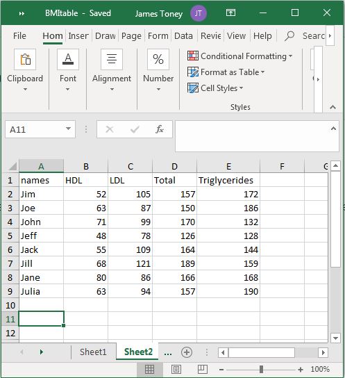
The data from this sheet can be read as follows:
>> cholesterolMatrix = readmatrix('BMItable.xlsx', 'Sheet', 2, 'Range', 'B2:E9')
cholesterolMatrix =
52 105 157 172
63 87 150 186
71 99 170 132
48 78 126 128
55 109 164 144
68 121 189 159
80 86 166 168
63 94 157 190
Or equivalently,
>> cholesterolMatrix = readmatrix('BMItable.xlsx', 'Sheet', 'Sheet2', 'Range', 'B2:E9')
There are numerous other qualifiers that can be used with this function to control how information is read from a file. See the MATLAB documentation for more details.
Checkpoint
An aside – readcell()
As shown in the examples above, readmatrix() can only read numerical data. To read text information from a spreadsheet, the function readcell() can be used. This function reads the data into a “cell array”, which is discussed in the next chapter. For completeness, an example of using this function is shown here. The NumHeaderLines qualifier directs MATLAB to skip the first row of the spreadsheet, which contains the column titles.
>> BMIcellArray = readcell('BMItable.xlsx', 'NumHeaderLines', 1)
BMIcellArray =
8×6 cell array
{'Jim' } {[70]} {[210]} {'M'} {[30.1286]} {'Obese' }
{'Joe' } {[72]} {[178]} {'M'} {[24.1385]} {'Normal' }
{'John' } {[68]} {[182]} {'M'} {[27.6700]} {'Overweight' }
{'Jeff' } {[65]} {[105]} {'M'} {[17.4710]} {'Underweight'}
{'Jack' } {[66]} {[142]} {'M'} {[22.9169]} {'Normal' }
{'Jill' } {[64]} {[121]} {'F'} {[20.7673]} {'Normal' }
{'Jane' } {[68]} {[152]} {'F'} {[23.1090]} {'Normal' }
{'Julia'} {[62]} {[172]} {'F'} {[31.4558]} {'Obese' }
The next chapter explains the notation and how to extract information from a cell array.
The converse of readmatrix() is writematrix(). If the function is called with only one argument – the variable name – the matrix is written to a text (ASCII) file that is named after the variable with the extension .txt. For example,
>> writematrix(cholesterolMatrix)
creates a text file called cholesterolMatrix.txt, containing the values from the matrix in comma-separated format:
>> type cholesterolmatrix.txt
52,105,157,172
63,87,150,186
71,99,170,132
48,78,126,128
55,109,164,144
68,121,189,159
80,86,166,168
63,94,157,190
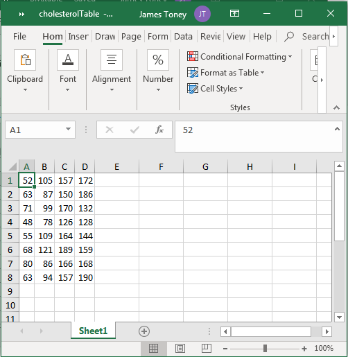
To write the data to a spreadsheet file, the filename (with the appropriate extension, such as .xlsx, .xls, .ods) is given as an argument; for example:
> writematrix(cholesterolMatrix, 'cholesterolTable.xlsx')
creates this file:
The sheet number or name and range of rows or columns can also be given as arguments, similarly to readmatrix(). See the documentation for more details.
Lecture Video 10.2 – Reading and Writing Spreadsheet Files
10.3 Reading and Writing General Text Files – fprintf() / fileread() / fgetl()
The load(), readmatrix() and writematrix() functions are most useful for data files with regular, row-by-column formats. For writing an arbitrary text file with a less regular structure, fprintf() is used; the syntax is exactly the same as writing to the command window, with 3 additions:
- The file must be opened using
fopen()prior to writing to it. - The file ID (which is returned by
fopen())is given as the first argument; a file ID of 1 means to write to the command window. - The file should be closed when writing is complete, using
fclose(). Otherwise, it may not be possible to open the file in other applications.
This example illustrates opening, writing, closing and typing a text file:
MATLAB users sometimes become confused about the difference between the file ID and the file name, and when to use each. Notice from the example that the file ID is just an integer – it is used instead of the file name when writing to and closing the file. Once the file is closed, the file ID no longer has meaning; therefore in the type command the file name is used.
To read the contents of a free-format text file, fileread() or fgetl() is used, depending on whether the objective is to read the file all at once or line-by-line. The fileread() function returns the entire contents of the file as a character array:
>> BMI_text = fileread('BMIoutput.txt')
BMI_text =
'Jim has a BMI of 30.1, so he is Obese
Joe has a BMI of 24.1, so he is Normal
John has a BMI of 27.7, so he is Overweight
Jeff has a BMI of 17.5, so he is Underweight
Jack has a BMI of 22.9, so he is Normal
Jill has a BMI of 20.8, so she is Normal
Jane has a BMI of 23.1, so she is Normal
Julia has a BMI of 31.5, so she is Obese
'
>>
This can be used as an alternative to the type command for displaying the contents of a text file. Notice that with fileread() it is NOT necessary to open the file prior to reading, and the file is specified by name.
The fgetl() function reads the file one line at a time; with this function, it IS necessary to open the file first. The function returns the next line of text as a character array; when the end of the file has been reached, it returns a value of -1. The next example shows how to read the text file line-by-line and pick out the name and weight classification from each entry. Note the use of the find() function to locate the blank spaces so that the name and weight classification can be extracted. There is an easier way, using the built-in function split(), but it relies on cell arrays, which are covered in the next chapter.
Lecture Video 10.2 – Writing General-Purpose ASCII Files
Checkpoint
10.4 File Selection Box
Rather than type in a file name, it is more convenient to browse for it, just as one normally does in Microsoft Office or other Windows or Mac applications. This can be done in a MATLAB programming using the function, uigetfile(). An example of its use is shown below:
>>file_name = uigetfile('*.xlsx')
(The argument in quotes is a filter; in this case, only files with the extension .xlsx will be displayed.) When this line is executed, a typical file selection box will open:
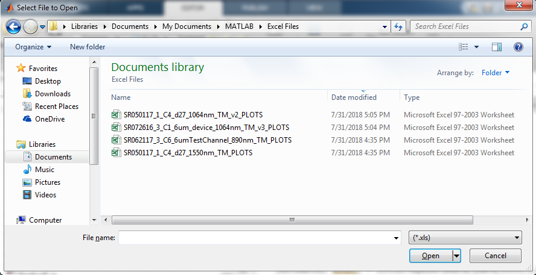
When the user selects a file and clicks open, the name of the file is stored in the variable, file_name. Note that this does not actually open the file – it is still necessary to use one of the file reading functions discussed earlier, like readmatrix() or fopen().
To enable browsing for a file across folders, a second output argument can be used to store the full path name. For example,
>> [file, path] = uigetfile('*.xlsx')
After the user navigates to the desired folder, selects a file and clicks Open, the file can be accessed by concatenating the path and file names, for example:
>> x = readmatrix([path, file]);
10.5 Problems
- Reading and Writing Files
a) Read columns B through F of the file test_scores.xlsx into a matrix called scores usingreadmatrix(). This will include NaNs for the first row, since the first row of the spreadsheet was non-numeric. DELETE THE FIRST ROW of scores – you should be able to do this with a single line of code, by assigning the first row of the array to [].
b) Read column A of the file test_scores.xlsx into a cell array called names usingreadcell(). This will include the column title, Students, in the cell array. If you are unfamiliar with cell arrays (covered in the next chapter), convert names to a string array:
names = string(names)
c) DELETE the first element of names, so that only the names themselves remain.
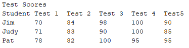
Write a text file in a nicely formatted table using fprintf(like the table shown below). The table should have an appropriate and clear title. Create column headers and label each row. Reminder: You must usefopen,fprintf, andfclose. You want to embed the student’s name followed by format conversion characters for the test scores for each student.
The text file should resemble this:
Find an error? Have a suggestion for improvement? Please submit this survey.
