13 Discrete-Time Simulation
Mathematics is an indispensable tool in engineering, but it is not always practical—or even possible—to obtain an exact solution to realistic problems. Increasingly engineers in all disciplines depend on numerical simulations to tackle problems that are not mathematically tractable. This chapter introduces basic techniques for numerical simulation, using MATLAB as the implementation platform. The objective is to present the key ideas rather than the most accurate or efficient techniques. Refer to textbooks on numerical analysis, differential equations or dynamic systems for a discussion of more sophisticated techniques.
13.1 Modeling of Physical Systems
A mathematical model is a set of equations that enables calculation of the behavior of an engineered or natural system. These equations are based on the underlying physics or chemistry of the system, but they are never a complete or exact description of the detailed processes. Consider, for example, the basic stress-strain equation ([latex]\sigma = Y \epsilon[/latex]). This macroscopic description in terms of Young’s modulus does not capture the microscopic details of the deformation of inter-atomic bonds. Yet it is a valid approach for determining the strain on members in structures, provided that certain simplifying assumptions are applicable. The most important assumption is that the stress is sufficiently small that only linear, elastic strain occurs. If that is not a valid assumption, then a more complex model must be used. However, engineers should always remember that no matter how detailed a model they construct, it is never exact. The guiding principle in determining how much complexity to incorporate into a model is that it should be as simple as possible while still permitting accurate determination of the key system characteristics.
13.1.1 Defining the System
The first step in creating a system model is to define the extent of the system being studied and its interactions with the rest of the world. As an example of constructing and simulating a model, consider a model of a hot water heater. A sensible choice of the system is the water tank, and its external interactions consist of:
- Cold water flowing into the tank
- Hot water flowing out of the tank
- Heat entering the tank from the heater
- Heat leaving the tank through the insulation
The second step in defining the model is to decide what quantities to use to describe the state of the system—these are called state variables. For the water heater example, a suitable set of state variables is the mass (M) of water in the tank and its temperature (T). Pressure could be added as a third state variable, but to keep the example simple, we will assume that the pressure is fixed.
A good practice is to draw a block diagram of the system showing the inputs, outputs and state variables, as shown in Figure 12.1. This type of diagram does not necessarily reflect the geometry of the system. By convention, inputs are normally shown on the left and outputs on the right, or top-to-bottom as with the heat flow.
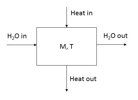
Figure 13.1: Diagram of a model of a hot water tank. M is the mass of water in the tank, and T is temperature.
The next step in developing the model is to write an equation or set of equations relating changes in the state variables (M and T in the water tank example) to the inputs and outputs. To keep the notation compact, a set of symbols is assigned to represent the inputs & outputs. The specific choice of symbols is arbitrary, but each engineering discipline typically has a conventional set of symbols. For the water tank example, we will use this set of symbols:[1]
Qin = input volume flow rate (volume per unit time)
Qout = output volume flow rate (volume per unit time)
Hin = heating rate (energy per unit time)
Hout = heat loss rate (energy per unit time)
In basic calculus terminology, the rate of change with time of a quantity, y, is the derivative, dy/dt or ẏ. Using this notation, the rates of change of T and M are:
[latex]\frac{dM}{dt} = \rho (Q_{in} - Q_{out})[/latex] (12.1)
[latex]\frac{dT}{dt} = \frac{(H_{in} - H_{out})}{C}[/latex] (12.2)
where [latex]\rho[/latex] is the density of water, which is needed to convert from volume to mass, and C is the heat capacity. This simplified set of equations neglects some effects, like the temperature dependence of C and the temperature difference between the inlet water and the water in the tank, that would be accounted for in a more accurate model.
These two equations are simple examples of differential equations—equations that are written in terms of derivatives of the dependent variables. In theory, equations (12.1a) and (12.1b) can be solved to give two functions of time, M(t) and T(t). There are a variety of techniques for solving differential equations analytically, but here we will focus on strictly numerical solutions.
13.1.2 Steady-State Solutions
Even without employing any complex mathematical methods or extensive calculations, it is often possible to predict the steady-state solution to a system of differential equations. The key idea is that if the inputs and outputs are fixed, eventually the system will stabilize at constant values of the state variables. At that point, the time derivatives are zero. Setting the time derivatives in (12.1 - 12.2) to zero results in
[latex]Q_{in} = Q_{out}[/latex] (at steady state)
[latex]H_{in} = H_{out}[/latex] (at steady state)
which leads to a fairly obvious conclusion: Steady state is reached when the inputs and outputs are balanced.
To extract useful information from this balance, we need more information: how the outputs depend on the state variables. The heat loss can be taken as proportional to the temperature difference between the inside and outside of the tank:
[latex]H_{out} = h (T - T_{0})[/latex]
where h is the heat transfer coefficient of the insulation and T0 is the ambient temperature, which is assumed to be fixed. For the case that no water is entering or leaving the tank, using this result leads to
[latex]H_{in} = h (T - T_{0})[/latex](at steady state)
which can be solved for the steady state temperature:
[latex]T = \frac{H}{h} + T_0[/latex] (at steady state)
This result shows that the steady-state temperature in the tank when it is idle (no water entering or exiting) can be calculated from the heating rate, heat transfer coefficient and ambient temperature.
Comparing the prediction of a simulation against the calculated steady-state solution is a valuable technique for validating the simulation method. Correctly predicting the steady-state solution does not guarantee that the simulation is correct, but failing to produce the correct steady-state solution guarantees that it is wrong.
13.2 From Differential Equations to Difference Equations
The objective in solving a differential equation is to go beyond the steady-state solution and determine how the state variables change with time. In this example, that means solving for M(t) and T(t). There are some cases in which the solution can be obtained in exact mathematical form, but there are others in which it is difficult or impossible to determine a closed-form solution. In those cases, numerical methods are needed. Although the water-heater problem described above is one that can be solved analytically, we will use it to illustrate a numerical approach.
The basic approach to numerical solution of differential equations is to replace the derivatives, e.g. dy/dt, by differences, e.g. [latex]\Delta y / \Delta t[/latex]. The differential equations are thus transformed into difference equations. The difference equation form of (12.1) and (12.2) is
[latex]\frac{\Delta M}{\Delta t} = \rho (Q_{in} - Q_{out})[/latex]
[latex]\frac{\Delta T}{\Delta t} = \rho (H_{in} - H_{out})[/latex]
The changes in the state variables in a time interval [latex]\Delta t[/latex] are then
[latex]\Delta M = \rho (Q_{in} - Q_{out}) \Delta t[/latex]
[latex]\Delta T = \frac{(H_{in} - H_{out})}{C} \Delta t[/latex]
The basic idea of a discrete-time simulation is to consider small increments of time, [latex]\Delta t[/latex], during which the inputs and outputs can be taken as constant. The changes in the state variables during that interval are calculated from the difference equations and added to the state variables. The quantity [latex]\Delta y[/latex] is the difference in the values of the variable y on two successive time steps:
[latex]y_{k+1} = y_k + \Delta y \Delta t[/latex]
where yk means the value of y on the kth time step. In the water tank example, the difference equations would be written as:
[latex]M_{k+1} = M_k +\rho (Q_{in} - Q_{out})\Delta t[/latex]
[latex]T_{k+1} = T_k + \frac{H_{in} - H_{out}}{C} \Delta t[/latex]
In MATLAB syntax, these difference equations could be written as
M(k + 1) = M(k) + rho*(Q_in - Q_out)*delta_t;
T(k + 1) = T(k) +(H_in - H_out)/C*delta_t;
Basic Algorithm for Discrete-Time Simulation
initialize the state variables
for each time step:
calculate the outputs (and inputs if necessary) based on the current values of the state variables
calculate the changes in the state variables based on those inputs and outputs
update the values of the state variables
repeat until simulation is complete
A key choice that must be made is the value of Δt. It is dictated by the time scale of the process being simulated—the appropriate time step may be pico- or nanoseconds in a circuit simulation, while it may be months or years in a population dynamics study. An essential requirement is that [latex]\Delta t[/latex] be small enough that the assumption of constant inputs and outputs during each time step is valid.
13.3 Discrete Time Simulation in Matlab
The following video gives a basic introduction to implementing a simulation in MATLAB.
(If the video does not load, try logging into ohiostate.pressbooks.pub in a separate tab, or try this direct link.)
The algorithm described above can be implemented in MATLAB using either a for loop (if the number of time steps is fixed) or a while loop (if the simulation is intended to run until some condition occurs). A simple program to simulate simultaneous filling and heating of the water tank is given below:
In this example the mass and temperature were treated as scalars, so that only the final values were stored. In many cases, it is desired to keep track of the entire history of the variables for later plotting and analysis. That issue is addressed in the next sub-section.
An unrealistic aspect of the program above is that it places no upper limit on the mass of water in the tank. A more realistic approach is to cut off the inflow when the capacity of the tank is reached using an if statement within the for loop, as shown here:
%Initialization section omitted for brevity
%Loop over all time steps
for t = 0: Dt : Nsteps*Dt %Calculate the heat loss based on the current temperature and mass
Hout = sigma*(T - T0); %Calculate the temperature change during this time step
DT = (Hin - Hout) / (M*C); %Calculate the mass change during this time step
%Only allow water to enter if the tank is not full
if M/rho < capacity
DM = rho*(Qin - Qout);
else
DM = 0;
end
%Update the state variables
M = M + DM;
T = T + DT;
end
A similar cutoff could be applied to prevent the temperature of the water from exceeding a specified maximum.
13.3.1 Organizing Simulation Data
The program above calculates the final mass and temperature but does not keep track of the intermediate values. In most cases it is useful to have a complete record of the state variables at all time steps. One way to do this is to create initially empty vectors called, for example, Tvec and Mvec, and append the latest T and M value to these vectors each time the loop is executed. That approach is shown here:
Appending values to the vectors during each execution of the loop is not the best practice in MATLAB, since re-allocating memory is a slow process. It is preferred, from a computational efficiency standpoint, to pre-allocate the storage for the row vectors when possible. One way to do this is to initialize them using the zeros() function. Within the loop, indexing is used to set the current values of Tvec and Nvec:
Tvec = zeros(1,Nsteps+1);
Mvec = zeros(1,Nsteps+1);
tvec = 0:Dt:Nsteps*Dt;
%Initialization section omitted for brevity
%Loop over all time steps
for tstep = 1: Nsteps+1
%Calculate the heat loss based on the current temperature and mass
Hout = sigma*(T - T0);
%Calculate the temperature change during this time step
DT = (Hin - Hout)*Dt / (M*C);
%Calculate the mass change during this time step
if M/rho < capacity
DM = rho*(Qin - Qout)*Dt;
else
DM = 0;
end
%Update the state variables
M = M + DM;
T = T + DT;
Tvec(tstep) = T;
Mvec (tstep) = M;
end
%Plotting section omitted for brevity – see previous example
13.4 Kinematics and Dynamic Systems
The technique described in the previous examples can be applied to any system that can be described by an ordinary differential equation. One important class of applications is kinematics – calculating the motion of a mechanical system, given its acceleration. The basic differential equations governing the motion of a particle are
[latex]\frac{dx}{dt} = v t[/latex]
[latex]\frac{dvx}{dt} = a t[/latex]
Where x(t),v(t), and a(t) are the position, velocity, and acceleration of the particle as a function of time. In the simplest approximation, known as the forward Euler method, the difference-equation approximations are written as:
[latex]x(t + dt) = x(t) + v(t) dt[/latex]
[latex]v(t + dt) = v(t) + a(t) dt[/latex]
The acceleration is determined by the specific physics of the problem. In general, it might depend on both the position and the velocity, as well as explicitly on time, so it can be expressed as
a(t)=f(x,v,t)
Important: the acceleration only depends on the current position, velocity and time. It does NOT depend on the prior acceleration. Thus the equation for a(t) is NOT a difference equation.
13.4.1 Constant-Acceleration Systems
The simplest type of kinematic problem is one in which the acceleration is constant. A common example is a free-falling object under the influence of gravity. Neglecting air resistance, and assuming the altitude is small relative to the radius of the planet, the acceleration is
a = -g
where for Earth, g = 9.81 m/s2 or 32.2 ft/s2. The minus sign simply indicates that the acceleration is downward. (Some people prefer to say that g = -9.81 m/s2, and a = g. Either convention is acceptable, so long as it is used consistently.)
The code to simulate a free-falling object that is thrown straight upward at an initial velocity, v0, starting from an initial height, y0 > 0, is shown below. In this case, the number of time steps is unknown – the simulation runs until the ball hits the ground. For that reason, a while loop is more appropriate than a for loop. Since the number of time steps is unknown, pre-allocation of memory for the arrays is not practical. In this example, we simply initialize them as scalars and append to them on each time step. This example uses a slightly different technique for appending to the arrays, using the end keyword.
Once the loop terminates – i.e. the simulation is complete, the height and velocity are plotted vs. time. Since they have different dimensions, they cannot be plotted on the same axes. In this example, a double-y-axis graph is used; subplots would be another option.
The previous program only works for y0 > 0. If y0 ≤ 0, the while loop will never execute – the condition must be modified to ensure that the program continues until the object reaches the ground on the way down, as shown below. That is the appropriate condition for this particular problem – for other problems, a different condition might be necessary.
%Initialization section omitted for brevity
%Loop until the object hits the ground on the way down
while y(end) > 0 || v(end) > 0
%Append new values of position, velocity, and time
y(end + 1) = y(end) + v(end) * dt;
v(end + 1) = v(end) - g * dt;
t(end + 1) = t(end) + dt;
end
%Plotting section omitted for brevity
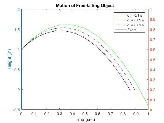
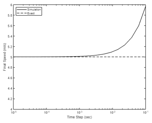
13.4.2 Effect of Time Step on Accuracy
As mentioned in Section 12.2, the time step, [latex]\Delta t[/latex], must be chosen carefully based on the physics of the problem. The free-fall problem is a good one to illustrate the effect of varying [latex]\Delta t[/latex], since the exact solution is known and can be used to judge the accuracy of the simulation.
The figure below shows the exact solution for y(t) compared to the simulation for several values of [latex]\Delta t[/latex]. As [latex]\Delta t[/latex] increases, the accuracy of the simulation degrades.
Another illustration of this effect is shown in the figure below, which plots the final speed of the object vs. [latex]\Delta t[/latex], compared to the exact result. This plot illustrates a characteristic of the forward Euler method – it tends to overestimate the velocity, creating the appearance of energy being added to the system, and this effect worsens as the time step is increased.
13.4.3 Variable-acceleration Systems: Drag, Thrust, and Universal Gravitation
Since the constant-acceleration problem can be solved exactly, using a discrete-time simulation is not really necessary, although these simple cases may be used for validation of a program. More complex problems, involving variable acceleration terms like drag and thrust, are more natural applications of simulation methods.
Drag is incorporated using the Newtonian model, in which the drag force is proportional to the square of velocity and always in the opposite direction from v. Mathematically this is expressed as
[latex]F_D = -\frac{1}{2}C_D\rho A v |v|[/latex]
where CD is the drag coefficient, [latex]\rho[/latex] is the density of air, and A is the cross-sectional area. The acceleration due to drag is calculated from Newton’s second law by dividing the drag force by the mass. In MATLAB code for a 1-D simulation, this can be implemented as
a_drag = -Cd*rho*A*abs(v)*v / m;
The example below incorporates drag into the previous free-falling projectile problem. Note that, because of the energy loss due to drag, the magnitude of the final velocity is lower than the initial velocity even though the initial and final heights are the same. Since the acceleration is not constant in this case, it is plotted along with the position and velocity in a 1x3 subplot.
The previous examples have all assumed that the acceleration due to gravity is constant, which is a reasonable approximation when the projectile is near the surface of Earth. For aeronautics problems, that assumption is not valid, and the more general expression based on Newton’s law of universal gravitation must be used:
[latex]g = -G \frac{M_{earth}} {(R_{earth} + y)^2}[/latex]
where Mearth is the mass of Earth, Rearth is its mean radius (assumed constant, although that is not strictly true) and y is the height of the object above the planet’s surface. Accounting for non-uniform gravity, the expression for the acceleration would be coded as
a(end + 1) = -(G*Mearth/(Rearth + y(end))^2 + … 1/2*rho*A*Cd*v(end)*abs(v(end))/m );
A further refinement that can be added is the variation of air density with altitude. One way of implementing that is to replace the constant rho by a call to a function that calculates the density based on altitude.
a(end + 1) = -(G*Mearth/(Rearth + y(end))^2 + … 1/2*air_density(y(end))*A*Cd*v(end)*abs(v(end))/m );
Another non-constant acceleration term is engine thrust. Engine thrust varies with pressure and therefore changes with altitude. Even if this effect is neglected, the engine may be on for only a portion of the flight, and it is necessary to keep track of which portions of the simulation have a non-zero thrust term. Further, the direction of the thrust may be opposite for take-off and landing phases. One way to implement this is with a variable, thrust_direction, that takes values of 1, 0, or -1 in the various phases of the flight (1=forward thrust, 0 = engine off, -1 = reverse thrust). Supposing that the thrust magnitude – assumed constant – is stored in a variable called Fthrust, the thrust term can then be incorporated as follows:
a(end + 1) = Fthrust*thrust_direction/m -(G*Mearth/(Rearth + y(end))^2 + … 1/2*air_density(y(end))*A*Cd*v(end)*abs(v(end))/m );
One last detail should be mentioned: since engines consume fuel and expel exhaust gases, the mass is not constant – it would be reduced in each time step according to the fuel burn rate whenever the engine is on.
13.5 Some Other Applications
The method illustrated in Sections 13.3 & 13.4 is applicable to any time-dependent ordinary differential equation. This section presents a few additional examples to demonstrate how the same basic approach can be applied to problems other than simple kinematics.
13.5.1 The Simple Pendulum
Consider the oscillation of a simple pendulum consisting of a point mass at the end of a massless rod of length l. The differential equation giving the angular acceleration,[latex]\theta[/latex], of the pendulum is:
[latex]\alpha = -g\ l\ sin\ \theta[/latex]
where g is the acceleration of gravity and l is the length of the pendulum. The angular velocity, [latex]\omega[/latex], and angular position, [latex]\theta[/latex], are calculated by the usual difference equations:
[latex]\theta_{k+1} = \theta_k + \omega_k \Delta t[/latex]
[latex]\omega_{k+1} = \omega_k + \alpha_k \Delta t[/latex]
The code to simulate the motion of the pendulum is essentially the same as the free-falling object, with a, v, and y being replaced by [latex]\alpha, \omega, and\ \theta[/latex]. The major difference is that the angular acceleration varies with [latex]\theta[/latex]. An example script to calculate the motion of a 0.5 m -long pendulum with an initial angle of [latex]\pi[latex]/6 radians (30o) and initial angular velocity of 0 is as follows. In addition to the simulation result, the analytical solution in the small-angle approximation ([latex]sin\ \theta \approx\theta[/latex]) is also calculated. From the plot, the divergence between the two is apparent, but in this case it is the “exact” solution that is wrong – the small-angle approximation is inaccurate for [latex]\theta[/latex] > 10o or so.
(More examples to be added.)
13.6 Conclusions
The examples presented in this chapter, while greatly simplified, were sufficient to illustrate the most important concepts and techniques of dynamic system modeling. The reader may already have anticipated effects that could be included in the model to make it more realistic. For example, in Section 13.1 the water entering the hot water tank is at a lower temperature than the water in the tank, so that the entering water would tend to reduce the temperature, but this effect was not accounted for in the model. If the inflow rate and the temperature difference between the inlet water and the tank are small, neglecting this effect might be justifiable. Otherwise, a more complex model might be necessary.
However, as mentioned in the opening paragraph of this chapter, no model is ever a complete and accurate description of a physical system. The complexity of a model should only be increased if doing so provides additional useful information about the system being simulated. A quote by the renowned statistician George Box makes this point: “All models are wrong, but some are useful.”
13.7 Problems
- A Bungee Jumper
%initial height in metersy = 1000; %acceleration of gravity in m/s^2g = 9.81;%spring constant in N/m, length of cord in mk = 20;L = 100;%mass of bungee jumper in kgm = 80;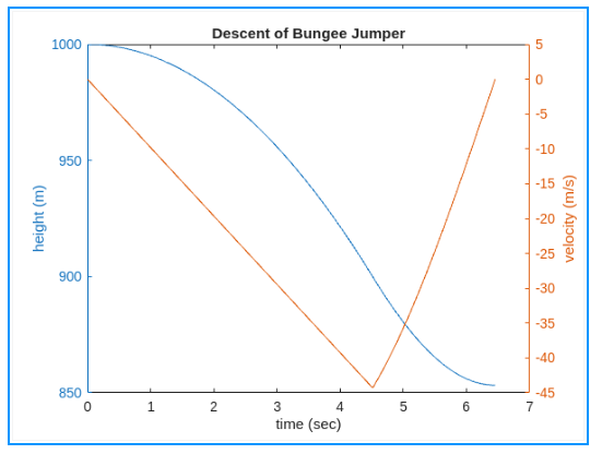
C_D = 0.8; %drag coefficientrho = 1.25; %density of airA = 0.5; %effective area%initial conditionsv = 0; %starts at rest at the top (beginning) of the inclinet = 0;s = 0;theta = pi/2; %incline is vertical at that point%parametersg = 9.81; %acceleration of gravity, m/s^2
R = 1.0; %radius of curvature, mmu_k = 0.25; %coefficient of kinetic friction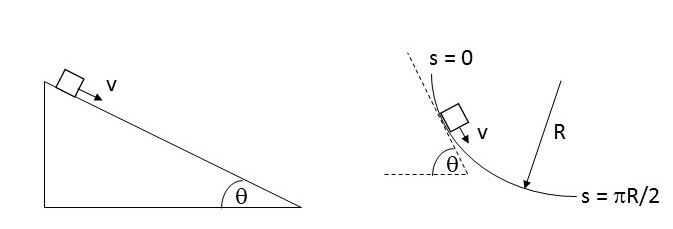
-
- Try validating your solution by setting the coefficient of friction to 0 and checking against conservation of energy. You will find a slight discrepancy, which should get smaller if you reduce the time step.
- What is the final value of θ? Does it make sense?
[latex]\\[/latex]
4. Damped Pendulum
A damped pendulum is shown in the figure:
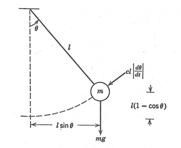
[latex]\alpha = -\frac{c}{ml}\omega-\frac{g}{l}\sin \theta\ = \frac{d\omega}{dt}[/latex]
c = 0.15;l = 0.5;g = 9.81;m = 0.2;k = 5;l = 1.5;g = 9.81;m = 2;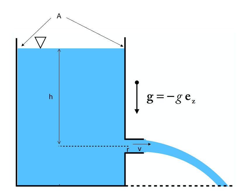
-
- The initial water level, h0
- the geometric parameters, A and r
-
- Initialize the velocity (v) based on the initial height (h0) using Equation (1)
- Until the water level is less than 0.001 times the initial level:
- Calculate the change in height, , based on the current velocity (v) using Equation (2)
- Update the h vector using the difference equation
-
- Update the velocity (v) based on the current height (h) using Equation (1)
-
- Print the time required for the tank to empty (regard the tank as empty when the water level is less than 0.001 times the initial level) to the command window.
A representative set of parameters is:
[latex]\\[/latex]
%Set geometric parametersr = 0.01; %radius of opening (m)A = pi; %tank area (m^2)g = 9.81; %acceleration of gravityh0 = 3.0; %initial water level (m)[latex]\\[/latex]
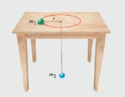
%physical parametersm1 = 0.1; %kgg = 9.81; %m/s^2mu_k = 0.01;m2 = 0.02; %kg
%initial conditionst = 0;v = 0; %m/sr = 0.2; %mtheta = 0;omega0 =sqrt(m2*g/(m1*r)); %with no friction, gives uniform circular motionpolarplot()) to plot the trajectory of m1 (r vs. θ). With the parameters above, it should look similar to this: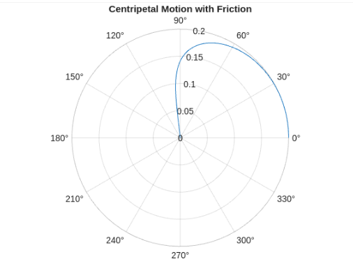
Find an error? Have a suggestion for improvement? Please submit this survey.
- This set of symbols is not by any means universal. Thermodynamics books often use Q for heat. ↵
