Module 3 Chapter 2: Quantitative Design Strategies

Previously, you reviewed different approaches to intervention and evaluation research and learned about a level of evidence (evidence hierarchy) model. These approaches and frameworks relate to how studies are designed to answer different types of research questions. The design strategies differ in the degree to which they address internal validity concerns—the ability to conclude that changes or differences can be attributed to an intervention rather than to other causes. Designs for quantitative intervention research are the focus of this chapter.

In this chapter, you learn about:

• pre-experimental, quasi-experimental, and experimental designs in relation to strength of evidence and internal validity concerns;
• how quantitative and single-system study designs are diagrammed;
• examples where different designs were used in social work intervention or evaluation research.

Addressing Internal Validity Concerns via Study Design Strategies

The study designs we examine in this chapter differ in terms of their capacity to address specific types of internal validity concerns. As a reminder of what you learned in our previous course, improving internal validity is about increasing investigator confidence that the outcomes observed in an experimental study are as believed, and are due to the experimental variables being studied. In the case of intervention research, the experimental variable being studied is the intervention.

Three general internal validity challenges are important to consider addressing with intervention research.

• Were there actually changes that occurred with the intervention (comparing participants’ status pre-intervention to their post-intervention status)?
• Did observed changes persist over time (comparing participants’ post-intervention status to their status at some later post-intervention follow-up time)?
• Is the observed change most likely due to the intervention itself?

Let’s consider how these three questions might relate to the kind of study design choices that investigators make.

Types of Intervention Research Designs

The intervention study design options can be loosely categorized into three types: pre-experimental, quasi-experimental, and experimental. Pre-experimental designs do not include comparison (control) groups, only the one group of interest. Quasi-experimental designs do include comparison (control) groups, but individuals are not randomly assigned to these groups—the groups are created naturally. Experimental designs include random assignment of study participants to the groups being compared in the study. These three types of designs differ in terms of their attempts to control as many alternative explanation factors as possible—the extent to which they address internal validity concerns.

Introducing short-hand for intervention study design diagrams.

It can become quite cumbersome to describe all the elements of an intervention study’s design in words and complete sentences; sometimes it is easier to use a diagram instead. This type of short-hand quickly communicates important information about a study design. It can become somewhat confusing, like understanding how the diagram of a football play drawn on a chalkboard translates into reality.

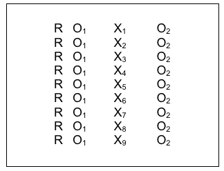
The first thing to know about this intervention study design short-hand is the symbols used and what each symbol means.

• X is used to designate that an intervention is being administered.
• [X] designates that an “intervention” or event naturally occurred, rather than one imposed by the investigator (for example, a change in policy, a natural disaster, or trauma-inducing crisis event).
• O is used to designate that an observation is being made (data are collected).
• Subscript numbers are used to designate which intervention or observation is relevant at that point. For example, X₁ might refer to the new intervention that is being tested and X₂ might refer to the second condition where the usual intervention is delivered. And, O₁ might refer to the first observation period (maybe before the intervention), O₂ to the second observation period (maybe after the intervention), and O₃ to a third observation period (maybe after a longer-term follow-up period).
• R is used to designate that individual elements were randomly assigned to the different intervention conditions. (Important reminder: This random assignment is not about random selection of a sample to represent a population; it is about using a randomization strategy for placing participants into the different groups in the experimental design).

Costs & Benefits of Various Design Strategies. 

Before we get into discussing the specific strategies that might be adopted for intervention research, it is important to understand that every design has its advantages and its disadvantages. There is no such thing as a single, perfect design to which all intervention research should adhere. Investigators are faced with a set of choices that must be carefully weighed. As we explore their available options, one feature that will become apparent is that some designs are more “costly” to implement than others. This “cost” term is being used broadly here: it is not simply a matter of dollars, though that is an important, practical consideration.

• First, a design may “cost” more in terms of more data collection points. There are significant costs associated with each time investigators have to collect data from participants—time, space, effort, materials, reimbursement or incentive payments, data entry, and more. For this reason, longitudinal studies often are more costly than cross-sectional studies.
• Second, “costs” increase with higher numbers of study participants. Greater study numbers “cost” dollars (e.g., advertising expenses, reimbursement or incentive payments, cost of materials used in the study, data entry), but also “cost” more in terms of a greater commitment in time and effort from study staff members, and in terms of greater numbers of persons being exposed to the potential risks associated with the intervention being studied.
• Third, some longitudinal study designs “cost” more in terms of the potential for higher rates of participant drop-out from the study over time. Each person who quits a study before it is completed increases the amount of wasted resources, since their data are incomplete (and possibly unusable), and that person may need to be replaced at duplicate cost.

Ten Typical Evaluation/Intervention Study Designs

This section presents 10 general study designs that typically appear in intervention and evaluation research. These examples are presented in a general order of increasing ability to address internal validity concerns, but this is offset by increasing costs in resources, participant numbers, and participant burden to implement. Many variations on these general designs appear in the literature; these are 10 general strategies.

#1: Case study.

Original, novel, or new interventions are sometimes delivered under unusual or unique circumstances. In these instances, when very little is known about intervening under those circumstances, knowledge is extended by sharing a case study. Eventually, when several case studies can be reviewed together, a clearer picture might emerge about intervening around that condition. At that point, theories and interventions can more systematically be tested. Case studies are considered pre-experimental designs.

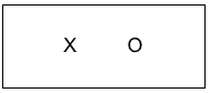
An example happened with an adolescent named Jeanna Giese at Milwaukee’s Children’s Hospital of Wisconsin. In 2004, Jeanna was bitten by a bat and three weeks later was diagnosed with full-blown rabies when it was too late to administer a vaccine. At the time, no treatments were known to be successful for rabies once it has developed; the rabies vaccine only works before the disease symptoms develop. Until this case, full-blown rabies was reported to be 100% fatal. The hospital staff implemented an innovative, theory and evidence-informed treatment plan which became known as the “Milwaukee Protocol.” The case study design can be diagrammed the following way, where X represents the “Milwaukee Protocol” intervention and O represents the observed outcomes of the treatment delivered in this case.

Jeanna Giese became the first person in the world known to survive full-blown rabies. The intervention team published the case study, and a handful of individuals around the world have been successfully treated with this protocol—rabies continues to be a highly fatal, global concern. The Milwaukee Protocol is considered somewhat controversial, largely because so few others have survived full-blown rabies even with this intervention being administered; some authors argue that this single case was successful because of unique characteristics of the patient, not because of the intervention protocol’s characteristics (Jackson, 2013).

This argument reflects a major drawback of case studies, which are pre-experimental designs: the unique sample/small sample size means that individual characteristics or differences can have a powerful influence on the outcomes observed. Thus, the internal validity problem is that the outcomes might be explained by some factors other than the intervention being studied. In addition, with a very small sample size the study results cannot be generalized to the larger population of individuals experiencing the targeted problem—this is an external validity argument. (We call this an “N of 1” study, where the symbol N refers to the sample size.) The important message here is that case studies are the beginning of a knowledge building trajectory, they are not the end; they inform future research and, possibly, inform practice under circumstances where uncertainty is high with very new problems or solutions. And, just in case you are curious: although some permanent neurological consequences remained, Jeanna Giese completed a college education, was married in 2014, and in 2016 became the mother of twins.

#2: Post-intervention only.

Looking a great deal like the case study design is a simple pre-experimental design where the number of individuals providing data after an intervention is greater than the single or very small number in the case study design. For example, a social work continuing education training session (the intervention) might collect data from training participants at the end of the session to see what they learned during the training event. The trainers might ask participants to rate how much they learned about each topic covered in the training (nothing, a little, some, a lot, very much) or they might present participants with a quiz to test their post-training knowledge of content taught in the session. The post-only design diagram is the same as what we saw with the single case study; the only difference is that the sample size is greater—it includes everyone who completed the evaluation form at the end of the training session rather than just a single case.

The post-intervention only design is cross-sectional in nature (only one data collection point with each participant). This design strategy is extremely vulnerable to internal validity threats. The investigator does not know if the group’s knowledge changed compared to before the training session: participants quizzed on knowledge may already have known the material before the training; or, a perception of how much they learned may not accurately depict how much they learned. The study design does not inform the investigators if the participants’ learning persisted over time after completing the training. The investigators also do not have a high level of confidence that the training session was the most likely cause of any changes observed—they cannot rule out other possible explanations.

In response to the internal validity threat concerning ability to detect change with an intervention, an investigator might ask study participants to compare themselves before and after the intervention took place. That would still be a simple post- only design because there is only one time point for data collection: post-intervention. This kind of retrospective approach is vulnerable to bias because it relies on an individual’s ability to accurately recall the past and make a valid comparison to the present, a comparison that hopefully is not influenced by their present state-of-mind. It helps to remember what you learned from SWK 3401 about the unreliability of the information individuals remember and how memories become influenced by later information and experiences.

#3: Pre-/Post- Intervention Comparison.

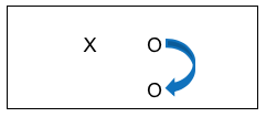
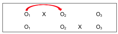
A wiser choice in terms of internal validity would be to directly compare data collected at the two points in time: pre-intervention and post-intervention. This pre-/post-design remains a pre-experimental design because it lacks a comparison (control) group. Because the data are collected from the same individuals at two time points, this strategy is considered longitudinal in nature. This type of pre-/post-intervention design allows us to directly identify change where observed differences on a specific outcome variable might be attributed to the intervention. A simple pre-/post- study design could be diagrammed like this:

Here we see an intervention X (perhaps our social work in-service training example), where data were still collected after the intervention (perhaps a knowledge and skills quiz). However, the investigators also collected the same information prior to the intervention. This allowed them to compare data for the two observation periods, pre- and post- intervention. See the arrow added to the diagram that shows this comparison:

While this pre-/post- intervention design is stronger than a post-only design, it also is a bit more “costly” to implement since there is an added data collection point. It imposes an additional burden on participants, and in some situations, it simply might not be possible to collect that pre-intervention data. This design strategy still suffers from the other two internal validity concerns: we do not know if any observed changes persisted over time, and we do not have the highest level of confidence that the changes observed can be attributed to the intervention itself.

#4: Pre-/Post-/Follow-Up Comparison.

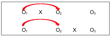
Investigators can improve on the pre-/post- study design by adding a follow-up observation. This allows them to determine whether any changes observed between the pre- and post- conditions persisted or disappeared over time. While investigators may be delighted to observe a meaningful change between the pre- and post- intervention periods, if these changes do not last over time, then intervention efforts and resources may have been wasted. This pre-/post-/follow-up design remains in the pre-experimental category, and would be diagrammed like this:

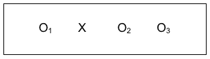
Here we see the intervention (X), with pre-intervention data, post-intervention data, and follow-up data being collected (O₁, O₂, and O₃). As an example, Wade-Mdivanian, Anderson-Butcher, Newman, and Ruderman (2016) explored the impact of delivering a preventive intervention about alcohol, tobacco and other drugs in the context of a positive youth development program called Youth to Youth International. The outcome variables of interest were the youth leaders’ knowledge, attitudes, self-efficacy, and leadership before the program, at the program’s conclusion, and six months after completing the program. The authors concluded that positive changes in knowledge and self-efficacy outcomes were observed in the pre-/post- comparison, though no significant change was observed in attitudes about alcohol, tobacco and other drugs; these differences persisted at the six-month follow-up. See the pre-/post-/follow-up design diagrammed with comparison arrows added:

This design resolved two of the three internal validity challenges, although at an increased cost of time, effort, and possibly other resources with the added data point. But an investigator would still lack confidence that observed changes were due to the intervention itself. Let’s look at some design strategies that focus on that particular challenge.

#5: Comparison Groups.

In our prior course we learned how to compare groups that differed on some characteristic, like gender for example. Comparison groups in intervention research allow us to compare groups where the difference lies in which intervention condition each received. By providing an experimental intervention to one group and not to the other group, investigator confidence increases about observed changes being related to the intervention. You may have heard this second group described as a control group. They are introduced into the study design to provide a benchmark for comparison with the status of the intervention group. The simplest form of a comparison group design, which is a quasi-experimental type of design, a post-only group design can be diagrammed as follows:

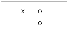
Consider the possibility in our earlier example of evaluating a social work training intervention that the team decided to expand their post only design to include collecting data from a group of social workers who are going to get their training next month. On the same day that the data were collected from the trained group, the team collected data from the untrained social workers, as well. This situation is a post-only design where the top row shows the group who received the training intervention (X) and the outcome was measured (O), and the bottom row shows the group without the training intervention (no X was applied) also being measured at the same point in time as the intervention group (O). This remains a cross-sectional study because each individual was only observed once. The following diagram shows the arrow where investigators compared the two groups on the outcome variables (knowledge and skills quiz scores, using our training example). If the training intervention is responsible for the outcome, the team would see a significant difference in the outcome data when comparing the two groups; hopefully in the direction of the trained group having better scores.

While this design has helped boost investigator confidence that the outcomes observed with the intervention group are likely due to the intervention itself, this post-only design “costs” more than a post-only single group (pre-experimental) study design. This post-only group design still suffers from a significant concern: how would an investigator know if the differences between the two groups appeared only after the intervention or could the differences always have existed, with or without the intervention? With this design, that possibility cannot be ignored. An investigator can only hope that the two groups were equivalent prior to the intervention. Two internal validity questions remain unanswered: did the outcome scores actually demonstrate a change resulting from intervention, and did any observed changes persist over time. Let’s consider some other combination strategies that might help, even though they may “cost” considerably more to implement.

#6: Comparison Group Pre-/Post- Design.

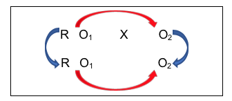
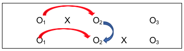
A giant leap forward in managing internal validity concerns comes from combining the strategy of having both an intervention and a comparison group (which makes it quasi-experimental) with the strategy of collecting data both before and after the intervention (which makes it longitudinal). Now investigators are able to address more of the major validity concerns. This comparison group pre-/post- design is diagrammed as follows:

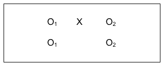
What the investigators have done here is collect data from everyone in their study, both groups, prior to delivering the intervention to one group and not to the other group (control group). Then, they collected the same information at the post-intervention time period for everyone in their study, both groups. The power in this design can be seen in the following diagrams that include arrows for the kinds of longitudinal pre-/post- comparisons that can be assessed, measuring change.

This is a pre-/post- comparison, indicating if change occurred with the intervention group after the intervention. Investigators would hope the answer is “yes” if it is believed that the intervention should make a difference. Similarly, the investigators could compare the non-intervention group at the two observation points (the lower arrow). Hopefully, there would be no significant change without the intervention.

You might be wondering, “Why would there be change in the no intervention group when nothing has been done to make them change?” Actually, with the passage of time, several possible explanatory events or processes could account for change.

• The first is simple maturation. Particularly with young children, developmental change happens over relatively short periods of time even without intervention.
• Similarly, the passage of time might account for symptom improvement even without intervention. Consider, for example, the old adage that, “if you treat a common cold it will take 7 to 10 days to get better; if you don’t treat it, it will take a week to a week-and-a-half.” Change without intervention is called spontaneous or natural change. Either way, there is change—with or without intervention.
• Third, given time, individuals in the no intervention group might seek out and receive other interventions not part of the study that also can produce change. This could be as simple as getting help and support from friends or family members; or, seeking help and advice on the internet; or, enrolling in other informal or formal treatment programs at the same time.

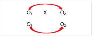
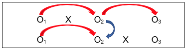
The benefit of combining the comparison groups and pre-/post- designs continues to emerge as we examine the next diagram showing comparisons an investigator can consider:

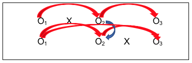
This group comparison of post-intervention results indicates whether there is a difference in outcomes between people who received the intervention and people who did not. Again, investigators would hope the answer is “yes,” and that the observed difference favors the intervention group. But with this design, an investigator can go even further in ruling out another possible explanation for outcome differences. Consider the power of this comparison:

By comparing the two groups BEFORE the intervention took place, an investigator can hopefully rule out the possibility that post-intervention group differences were actually a reflection of pre-existing differences; differences that existed prior to the intervention. In this case, the investigator would hope to observe no significant differences in this comparison. This “no differences” result would boost confidence in the conclusion that any observed post-intervention differences were a function of the intervention itself (since there were no pre-existing differences). Not being able to rule out this possibility was one limitation of the post-only group comparison strategy discussed earlier.

A Note About Non-Treatment, Placebo, and Treatment as Usual Comparison Groups.

What we have diagrammed above is a situation where the second group received no treatment at all. This, however, is problematic in three ways. First, the ethics of intentionally not serving individuals who are seeking help with a social work problem is concerning. Second, the scientific integrity of such studies tends to suffer because non-treatment “control” groups tend to have high rates of study drop out (attrition) as those participants seek help elsewhere. Third, the results of these studies are coming under great scrutiny as the world of behavioral science has come to realize that any treatment is likely to be better than no treatment—thus, study results where the tested intervention is significantly positive may be grossly over-interpreted. Compared to other treatments, what appears to be a fantastic innovation may be no better.

Medical studies often include a comparison group who receives a “fake” or neutral form of a medication or other intervention. In medicine, a placebo is an inert “treatment” with a substance that has no likely known effect on the condition being studies, such as a pill made of sugar, for example. The approximate equivalent in behavior al science is an intervention where clients are provided only with basic, factual information about the condition; nothing too empowering. In theory, neither the placebo medication nor the simple educational materials are expected to promote significant change. This is a slight variation on the non-treatment control condition. However, over 20 years of research provided evidence of a placebo effect that cannot be discounted. In one systematic review and meta-analysis study (Howick et al, 2016) the size of effect associated with placebos were no different or even larger than treatment effects. This placebo effect is, most likely, associated with the psychological principles of motivation and expectancies—expecting something to work has a powerful impact on behavior and outcomes, particularly with regard to symptoms of nausea and pain (Cherry, 2018). Of course, this means that participants receiving the placebo believe they are (or could be) receiving the therapeutic intervention. Also interesting to note is that participants sometimes report negative side-effects with exposure to the placebo treatment.

In medication trials, the introduction of a placebo may allow investigators to impose a double-blind structure to the study. A double-blind study is one where neither the patient/client nor the practitioner/clinician knows if the person is receiving the test medication or the placebo condition. The double-blind structure is imposed as means of reducing practitioner bias in the study results from either patient or practitioner/clinician beliefs about the experimental medication. However, it is difficult to disguise behavioral interventions from practitioners—it is not as simple as creating a real-looking pill or making distilled water look like medicine.

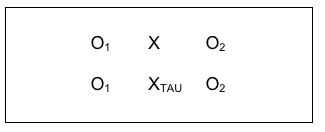
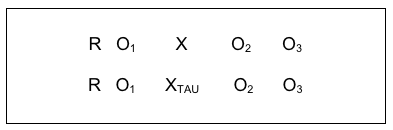
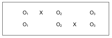
More popular in intervention science today is the use of a treatment as usual condition (TAU). In a TAU study, the comparison group receives the same treatment that would have been provided without the study being conducted. This resolves the ethical concerns of intentionally denying care to someone seeking help simply to fulfill demands of a research design. It also helps resolve the study integrity concerns mentioned earlier regarding non-treatment studies. But this design looks a little bit different from the diagram of a comparison group design. You will notice that there is a second intervention “X” symbol in the diagram and that the new X has a subscript notation (TAU) so you can tell the two intervention groups apart, X and X_TAU.

#7: Single-System Design.

A commonly applied means of evaluating practice is to employ a quasi-experimental single-system design. This approach uniquely combines aspect of the case study with aspects of the pre-experimental pre-/post-design. Like the case study, the data are collected for one single case at a time—whether the element or unit of study is an individual, couple, family, or larger group, the data represent the behavior of that element over time. In that sense, the single-system design is longitudinal—repeated measurements are drawn for the same element each time. It is a quasi-experimental design in that conditions are systematically varied, and outcomes measured for each variation. This approach to evaluating practice is often referred to as a single-subject design. However, the fact that the “subject” might be a larger system is lost in that label, hence a preference for the single-“system” design label.

The single-system design is sufficiently unique in implementation that an entirely different notation system is applied. Instead of the previous Xs and Os, we will be using A’s and B’s (even C’s and D’s). The first major distinction is that instead of a pre-intervention measurement (what we called O₁) we need a pre-intervention baseline. By definition, a line is the distance between two or more points, thus in order to be a baseline measurement, at least two and preferably at least 7 pre-intervention measurement points are utilized. For example, if the target of intervention with a family is that they spend more activity time together, a practitioner might have them maintain a daily calendar with the number of minutes spent in activity time is recorded for each of 7 days. This would be used as a baseline indication of the family’s behavioral norm. Thus, since there are 7 measurement points replacing the single pre-intervention observation (O₁), we designate this as A₁, A₂, A₃ and so forth to A₇ for days 1 through 7 during the baseline week–this might extend to A₃₀ for a month of baseline recording.

Next, we continue to measure the target behavior during the period of intervention. Because the intervention period is different from the baseline period, we use the letter B to indicate the change. This corresponds to the single point in our group designs where we used the letter X to designate the intervention. Typically, in a pre-/post- intervention study no data are collected during the intervention, X, which is another difference in single-system designs. Let’s say that the social worker’s intervention was to text the family members an assigned activity for each of 10 days, and they continued to record the number of minutes when they were engaged in family activity time each day. Because it is a series of measurement points, we use B₁, B₂, B₃ and so forth for the duration of the intervention, which is B₁₀ in this case. The next step is to remove the daily assignment text messages, giving them just one menu on the first of the next 7 days, from which the family is expected to pick an activity and continue to record time spent in family activity time each day. This would be a different form of intervention from the “B” condition, so it becomes C₁, C₂, C₃, and so forth to the end, C₇. Finally, the social worker no longer sends any cues, and the family simply records their daily family activity time for another week. This “no intervention” condition is the same as what happened at baseline before there was any intervention. So, the notation reverts back to A’s, but this time it is A₈, A₉, A₁₀, and so forth to the end of the observation period, A₁₄. For this reason, single system design studies are often referred to as “ABA” designs (initial baseline, an intervention line, and a post-intervention line) or, in our example an “ABCA” design since there was a second intervention after the “B” condition. This single-system design notation is different from the notation using Xs and Os because data are collected multiple times during each phase, rather than at each single point during pre-intervention, intervention, and post-intervention.

The data could be presented in a table format, but a visual graph depicts the trends in a more concise, communicative manner. What the practitioner is aiming to do with the family is to look at the pattern of behavior in as objective manner as possible, under the different manipulated conditions. Here is a graphical representation from one hypothetical family. As you can see, there is natural variation in the family’s behavior that would be missed if we simply used a single weekly value for the pre- and post-intervention periods instead.

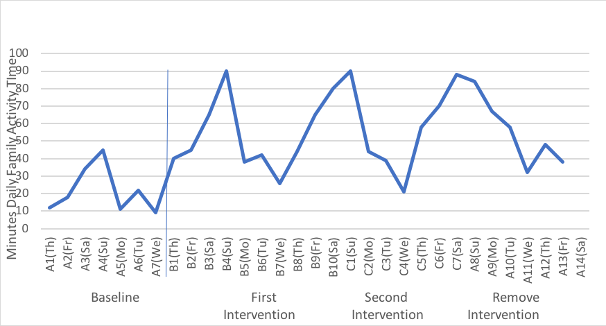
Together, the practitioner and the client family can discuss what they see in the data. For example, what makes Wednesday family activity time particularly difficult to implement and does it matter given the what happens on the other days? How does it feel as a family to have the greater activity days, and is that rewarding to them? What happens when the social worker is no longer prompting them to engage in activities and how can they sustain their gains over time without outside intervention? What new skills did they learn that support sustainability? What will be their cue that a “booster” might be necessary? What the data allow is a clear evaluation of the intervention with this family, which is the main purpose of practice evaluation using the single-system design approach.

#8: Random Control Trial (RCT) Pre-/Post- Design.

The major difference between the comparison group pre-/post- design just discussed and the random control trial (RCT) with pre-/post- design is that investigators do not have to rely so much on hoping that the two comparison groups were initially equivalent: they randomly assign study participants to the two groups as an attempt to ensure that this is true. There is still no guarantee of initial group equivalence; this still needs to be assessed. But the investigators are less vulnerable to the bad luck of having the two comparison groups being initially different. This is what the RCT design looks like in a diagram:

Many authors of research textbooks describe the RCT as the “gold standard” of intervention research design because it addresses so many possible internal validity concerns. It is, indeed, a powerful experimental design. However, it is important to recognize that this type of design comes at a relatively high “cost” compared to some of the others we have discussed. Because there are two comparison groups being compared, there are more study participant costs involved than the single group designs. Because there are at least two points in time when data are collected, there are more data collection and participant retention costs involved than the single time point post-only designs. And random assignment to experimental conditions or groups is not always feasible in real-world intervention situations. For example, it is difficult to apply random assignment to conditions where placement is determined by court order, making it difficult to use an RCT design for comparing a jail diversion program (experimental intervention) with incarceration (treatment as usual control group). For these practical reasons, programs often settle on group comparison designs without random assignment in their evaluation efforts.

A slight variant on this study design was used to compare a screening and brief intervention (SBI) for substance misuse problems to the usual (TAU) condition among 729 women preparing for release from jail and measured again during early reentry to community living (Begun, Rose, & LeBel, 2011). One-third of the women who had positive screen results for a potential substance use disorder were randomly assigned to the treatment as usual condition (X_TAU), and two-thirds to the SBI experimental intervention condition (X) as diagrammed below. The investigators followed 149 women three months into post-release community reentry ( follow-up observation), and found that women receiving the innovative SBI intervention had better outcomes for drinking and drug use during early reentry (three months post-release): the mean difference in scores on the AUDIT-12 screening instrument prior to jail compared to reentry after release was more than 5 points (see Back to Basics Box for more details). The random controlled trial with pre/post/follow-up study design looked like this:

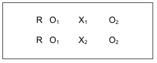
#9: Random Control Trial (RCT) Comparing Two (or More) Interventions.

The only difference between the design just discussed and the random control trial that compares two interventions is the indicator associated with the intervention symbol, X. The X₁ and X₂ refer to two different interventions, the same way the X₁ and X_TAU reflected two different intervention conditions above. This kind of design is used to determine which of two interventions has greater effectiveness, especially if there is a considerable difference in cost of delivering them. The results can help with a cost-benefit comparison which program administrators and policy decision-makers use to help make decisions about which to fund. It is possible to compare more than two interventions by simply adding additional lines for each group (X₃, X₄, and so on). Each group added, however, also adds considerably to the “costs” of conducting the study.

The COMBINE Project was an historic example where multiple intervention approaches were compared for their effectiveness in treating alcohol dependence (see NIAAA Overview of COMBINE at https://pubs.niaaa.nih.gov/publications/combine/overview.htm).

Two medications were being compared (acamprosate and naltrexone) along with medical management counseling for adherence to the medication protocol (MM), and medication with MM was compared to medication with MM plus a cognitive behavioral psychotherapy intervention (CBI). Clients were randomly assigned to 9 groups with approximately 153 clients per group:

X₁-acamprosate placebo + naltrexone placebo + MM (no CBI)

X₂-acamprosate + naltrexone placebo + MM (no CBI)

X₃-naltrexone + acamprosate placebo + MM (no CBI)

X₄-acamprosate + naltrexone + MM (no CBI)

X₅– acamprosate placebo + naltrexone placebo + MM + CBI

X₆– acamprosate + naltrexone placebo + MM + CBI

X₇– naltrexone + acamprosate placebo + MM + CBI

X₈– acamprosate + naltrexone + MM + CBI

X₉-no pills or MM, CBI only

The COMBINE Project was an extremely “costly” study to conduct given the number of study participants needed to meet the study’s design demands–one reason why it was a collaboration across multiple study sites. The results included participants in all 9 groups showing at least some improvement as measured by a reduction in drinking–intervention is almost always an advantage over no intervention. The poorest results were observed for the last group (X₉), those receiving the specialty cognitive behavioral intervention (CBI) alone, with no medication or placebo medication. Surprising was that best outcomes were observed for the group receiving CBI with both placebo medications and medication management (MM) counseling (X₅)! The other group with best outcomes was the group receiving naltrexone with MM counseling but no CBI (X₃). The investigative team concluded that pharmacotherapy combined with medication counseling can yield clinically significant alcohol treatment outcomes, and this can be delivered in primary care settings where specialty alcohol treatment is unavailable (Pettinati, Anton, & Willenbring, 2006). They were surprised, also, by the lack of observed advantage to using the medication acamprosate because it had so much evidence support from studies conducted in European countries. This map of the design does not show the multiple follow-up observations conducted in the study.

#10: Comparison Group with a Delayed Intervention Condition.

One way of overcoming the ethical dilemma of an intervention/no intervention study design is to offer the intervention condition later for the second group. Not only does this more evenly distribute risks and benefits potentially experienced across both groups, it also makes sense scientifically and practically because it allows another set of comparison conditions to be longitudinally analyzed for a relatively smaller additional “cost.” Here is what this design strategy might look like using our study design notation:

Look at all the information available through this design:

• First is a simple pre-/post- design (O₁ to O₂ with X), where investigators hope to see a difference;
  
• Second is the control group pre-/post- comparison (O₁ to O₂ without intervention X), where investigators hope for no difference, or at least significantly less difference than for the group with the intervention early on;
  
• Third is the comparison of the group with the intervention (X) to the group without the intervention, after the intervention was delivered (O₂ for each group), where the investigators hope to see a significant difference between the two groups, and that the difference favors the group who received the intervention (X);
  
• Fourth is the post-/follow-up comparison for the group with the intervention (O₂ to O₃), where investigators hope that the changes seen on O₂ persisted at O₃ (or are even more improved, not that they declined over time;
  
• Fifth is the ability to replicate the results of the first group receiving the intervention with the results for the second group to receive the intervention (O₂ for the first group with O₃ for the second group—actually, change from O₁ to O₂ for the first group and change from O₁ to O₃ for the second group). Ideally, the investigators would see similar results for the two groups—those who received the intervention early on and those who received it a bit later;
  
• Sixth is the ability to test the assumption that the two groups were similar prior to the study beginning—that the differences observed between them were related to the intervention and not pre-existing group differences (O₁ for both groups), as well as differences immediately after intervention and between follow-up and immediately post-intervention.
  

This study design was used to examine the effectiveness of equine-assisted therapy for persons who have dementia (Dabelko-Schoeny, et al., 2014). The study engaged 16 participants with Alzheimer’s Disease in activities with four horses (grooming, observing, interacting, leading, and photographing). Study participants were randomly assigned to two groups: one received the intervention immediately the other did not; however, this latter group received the intervention later, after the intervention was withdrawn from the first group. When not receiving the equine-assisted therapy, participants received the usual services. Thus, the investigators were able to make multiple types of comparisons and ensured that all participants had the opportunity to experience the novel intervention. The team reported that the equine-assisted therapy was significantly associated with lower rates of problematic/disruptive behavior being exhibited by the participants in their nursing homes and higher levels of “good stress” (sense of exhilaration or accomplishment) as measured by salivary cortisol levels.

Major disadvantages of this study design:

• it may be that social work interventions are best delivered right away, when the need arises, and that their impact is diminished when delivered after a significant delay;
• the design is costlier to implement than either design alone might be, because it requires more participants and that they be retained over a longer period of time.

Chapter Conclusion

As you can see, social work professionals and investigators have numerous options available to them in planning how to study the impact of interventions and evaluate their practices, programs, and policies. Each option has pros and cons, advantages and disadvantages, costs and benefits that need to be weighed in making the study design decisions. New decision points arise with planning processes related to study measurement and participant inclusion. These are explored in our next chapters.

Stop and Think