Module 4 Chapter 1: Review and Extension of Descriptive and Group Comparison Analyses
In our previous course you learned to distinguish between univariate and bivariate analyses, and to both conduct and interpret a variety of each type of analysis. Those activities were directed toward evidence for understanding diverse populations, social work problems, and social phenomena. Much of what was learned applies to our current course concerned with intervention and evaluation research for understanding social work interventions. In this chapter, these concepts will be reviewed in the context of intervention and evaluation research.
In this chapter you:
- review principles of univariate analysis (mean, median, and standard deviation), this time as applied to data for understanding social work interventions;
- review principles of bivariate analysis (single sample t-test, independent samples t-test, analysis of variance, chi-square, and non-parametric analytic approaches), this time as applied to data for understanding social work interventions;
- learn basic principles about logistic regression which can answer questions about dichotomous intervention outcomes.
Review of Univariate Statistics Extended to Intervention Research
In our previous course (Module 4, Chapter 2), you learned about analyses that describe data one, single variable at a time—univariate analysis. These descriptive statistics and analyses continue to be relevant in research for understanding social work interventions:
- Frequency & proportion data (categorical variables)
- Central tendency analysis (numeric/continuous variables)
- mean
- median
- mode
- Distribution analysis (numeric/continuous variables)
- range
- variance
- standard deviation
- normal curve
- skew & kurtosis
For example:
- In evaluating an intervention to help families who are or at risk of homelessness, you might collect and analyze data concerning the proportion of families who were able to achieve stable housing status for a year or more (a dichotomous, categorical variable).
- You might wish to compare the mean number of disciplinary actions that occur in middle school classrooms before and after teachers are trained to employ trauma-informed teaching and classroom management practices.
- In evaluating the impact of an intervention on native-speakers of English with its impact on individuals for whom English is a second or third language, you might examine the variance in outcomes for these two groups—little variability in the second group might indicate that the intervention was not being adequately “received” or “processed” by these individuals.
- You may need to assess the distribution of values on an outcome variable in planning your statistical analyses in an intervention study—whether or not the values are relatively normally distributed may determine which statistical tests are most appropriate.
Review of Bivariate Analysis Extended to Intervention Research
Recall that bivariate analysis is about assessing the nature and strength of relationships that exist between two variables. In our previous course you learned several statistical tests for answering different types of research questions using different types of variables. You learned about the:
- single sample t-test
- independent samples t-test
- analysis of variance (Anova)
- chi-square test
- correlation test
In evaluating social work interventions, any of these tests might be applied, depending on the nature of the study questions, study design, and study variables involved. Here we will review all but the correlation test because that it seldom used as a means of evaluating outcomes in intervention research.
Single sample t-test.
In a very simple post-only study design an investigator might wish to compare a group’s mean outcome score to a pre-determined, established standard or norm value. This would be used, for example, to evaluate the impact of an intervention to improve the health of infants born to mothers who smoke cigarettes by reducing or eliminating smoking during pregnancy (and, ideally, after birth, as well). The outcome measure could be the newborn infants’ 5-minute Apgar scores, a measure routinely recorded at birth for all babies born in the United States (and many other countries). An Apgar score of 7, 8, or 9 means an infant is healthy; lower Apgar scores are associated with poorer health outcomes. Apgar scores can only be measured within minutes following birth, so a post-only design might make sense. The null hypothesis would be:
H0: the post-intervention mean Apgar score (measured at 5-minutes post-birth) is 7 or greater for babies born to mothers who received the intervention.
You can refer to your prior course Excel workbook exercises as a reminder of how to implement the steps involved in a single sample t-test. The selection of 7 as the comparison mean value is a bit arbitrary. Ideally, the investigators have historical data from before the intervention was made available concerning the mean 5-minute Apgar score for mothers who smoke. For now, the investigation uses the “healthy baby” value as the comparison mean.

Independent samples t-test.
In Module 3 we considered study designs for answering research questions that involve comparing two intervention conditions. This might be a new intervention being compared to no intervention, a placebo, or a treatment-as-usual (TAU) “control” condition. Once investigators have collected outcome data for study participants who are exposed to these different intervention conditions, it is time to analyze those data to see if the hypothesized differences between the groups are actually observed. This is identical to the use of independent samples t-tests examined in our prior course where they were used to answer questions comparing groups to answer questions about diverse populations, social work problems, or social phenomena. Recall that certain assumptions need to be fulfilled in order to use this test—assumptions related to normal distribution and variance equality, for example. Otherwise, non-parametric analyses would be preferable. For the sake of clarity, let’s work with a specific example using independent samples t-tests to evaluate an intervention.
A Canadian team of investigators (Toneatto, Pillai, & Courtice, 2014) wanted to know if an intervention that enhanced Cognitive Behavioral Therapy (CBT) for problem gambling with Mindfulness Training was better than no intervention (the control group participants were on a wait-list for the program and did, eventually, receive the intervention). Both groups in this pilot study (N=18 participants total, 9 in each group) were measured before and after the intervention. The study design looked like this (note there was no random assignment to the intervention or wait-list control condition):
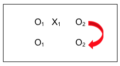
The Variables.
In this example, the observation (O2) data reflect the outcome variable. In this case, the outcome variables were expected to be dependent on the intervention condition manipulated by the investigators: Mindfulness Enhanced Cognitive Behavioral Therapy (M-CBT) versus Wait List Control (no intervention). Thus, the outcome variables are the dependent variables in this example. The outcome variables were a set of measures of gambling urges and symptoms; we can demonstrate the important points with just two of these, gambling diagnosis symptoms and gambling urges. Both of these variables are numeric in nature, with the scale on each showing that a higher score means a more serious gambling problem.
The Null Hypothesis.
The research question being asked is if there existed a significant difference between the outcomes for the group receiving the experimental intervention (X1) and the group on the waiting list (non-treatment control)—was the difference between these two groups meaningfully different from zero (no difference)? In statistics logic, the investigators were testing the null hypothesis that the difference between the two groups was zero.
H0: there exists no statistically significant difference in symptoms or craving outcomes for the two treatment groups.
If the results of analysis led the investigators to reject the null hypothesis, it means they were reasonably confident that there existed a meaningful difference between the two groups (the difference was NOT zero). If the analysis led the investigators to fail to reject the null hypothesis, it means that no difference was detected (but they cannot conclude that no difference exists).
The Statistical Analysis Approach.
Since exactly two groups were compared, the independent groups t-test was appropriate. (Remember, in our prior course you learned that if three or more groups were being compared, an analysis of variance would be required; if only one group was involved, a single-sample t-test would be appropriate.) The underlying assumptions for this type of analysis are exactly the same as what you learned in in our prior course:
- Type of (Outcome) Variable: The scale of measurement for the dependent variable is continuous (interval).
- Normal Distribution: The dependent variable is normally distributed in the population, or a sufficiently large sample size was drawn to allow approximation of the normal distribution. Note: the “rule of thumb” is that neither group should be smaller than 6, and ideally has more.
- Independent Observations: Individuals within each sample and between the two groups are independent of each other—random selection indicates that the chances of any one “unit” being sampled are independent of the chances for any other being sampled.
- Homogeneity of Variance: Variance is the same for the two groups, as indicated by equal standard deviations in the two samples.
The independent groups t-test analysis (sometimes called a student’s t-test) involved dividing a difference score by a variance estimate. This is accomplished by the following steps:
- calculating the mean score for each group (2 groups’ means are called Mgroup1 and Mgroup2);
- computing a “difference from the mean” score for each individual participant in each of the 2 groups—this is called the deviation score for each participant—then squaring that deviation score for each participant in each of the 2 groups;
- computing the sum of the squared deviation scores for each group;
- calculating the estimate for variance as the standard deviation squared for each group (Sgroup12 and Sgroup22) by taking the sum of the squared deviation scores for each group calculated in step 3 and dividing by the number of cases in that group minus 1 (ngroup1 – 1 and ngroup2 – 1 );
- compute the t-value as the difference between the two groups’ means (this is Mgroup1– Mgroup2) divided by the square root of a variance estimate computed as [(Sgroup12 divided by ngroup1) + (Sgroup22 divided by ngroup2);
- compare the computed t-value with the criterion value identified using the degrees of freedom for the total N-2 (where N is the total number of participants in the two groups combined) and the α<.05 criterion.
Here is how it worked out in our example about the gambling intervention.
The Analysis Results and Interpretation.
The investigators observed a statistically significant difference in both outcome variables when they compared the enhanced intervention group to the non-treatment (wait listed) control group. Furthermore, the difference was in the expected direction: the intervention group’s mean scores were lower, indicating less severe gambling symptoms, than the control group’s mean scores.
Table 1. Outcome measures by group (adapted from Toneatto et al, 2014).
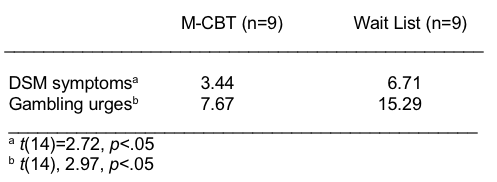
For both study outcome measures (symptoms and urges), the differences between the two treatment group means were statistically significant (the p<.05). Thus, the investigators rejected the null hypothesis of no difference (that the difference was zero) and concluded that mindfulness enhancement of cognitive behavioral therapy for problem gambling warrants further, more systematic research attention. One caution about over-interpreting these results is that intervention of any type is usually preferable to no treatment; future research should compare the mindfulness enhancement to the treatment-as-usual condition or the cognitive behavioral therapy alone.
Remember, also, that a strong intervention or evaluation research study also includes information concerning effect sizes—not only whether the differences were statistically significant but were they of meaningful magnitude, were the differences clinically significant?

Analysis of variance (Anova).
The independent samples t-test is a fine analysis when two groups are compared. But, as you learned in our prior course, analysis of variance (Anova) is preferred when more than two groups are being compared. Again, recall that certain assumptions need to be fulfilled in order to use this test—assumptions related to normal distribution and variance equality, for example. Otherwise, non-parametric analyses would be preferable. Consider the example presented by Walsh and Lord (2004) in their study of client satisfaction with social work services. In one analysis, the authors compared satisfaction scores for three groups of parents referred for social work services in a pediatric hospital setting. The three groups were:
- parents referred for practical assistance(X1)
- parents referred for counselling (X2)
- parents referred for both practical assistance and counselling (X3)
A diagram of this scenario might look like this:
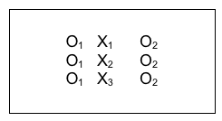
The Variables.
In this example, the observation (O2) data reflected the outcome (dependent) variable—client satisfaction. Client satisfaction was numeric in nature with higher scores indicating greater satisfaction. The investigators wondered if this was dependent on the parents’ referral—a 3-category categorical variable.
The Null Hypothesis.
The research question asked was if there existed a significant difference between the outcomes (client satisfaction) for parents referred only for practical assistance (n=4), only for counseling (n=9), and for both practical assistance and counseling (n=6). In statistics logic, the investigators were testing the null hypothesis that the difference between the three groups was zero.
H0: There exists no statistically significant difference in client satisfaction between these three groups of parents.
If the results of analysis led the investigators to reject the null hypothesis, it means they could be reasonably confident that there existed a meaningful difference between at least two groups, but they would not know which two groups without conducting further analyses. For example the difference(s) could be between:
- X1 and X2
- X1 and X3
- X2 and X3
- X1 and X2 and X3.
The Anova test would be called an omnibus test of significance, meaning that it covers the whole group of possible comparisons, and the investigators would follow up with post hoc analyses to determine where the differences actually lie.
The Statistical Analysis Approach.
Since more than two groups were compared, the analysis of variance (Anova) test should have been appropriate—but there is a problem with the sample size (see the assumptions list below). The underlying assumptions for this type of analysis are exactly the same as what you learned in in our prior course:
- Type of (Outcome) Variable: The scale of measurement for the dependent variable is numeric or continuous (interval).
- Normal Distribution: The dependent variable is normally distributed in the population, or a sufficiently large sample size was drawn to allow approximation of the normal distribution. Note: the “rule of thumb” is that no group should be smaller than 6, and ideally has more. In our example, this assumption was violated—the groups were as small as 4, 6, and 9.
- Independent Observations: Individuals within each sample and between the two groups are independent of each other—random selection indicates that the chances of any one “unit” being sampled are independent of the chances for any other being sampled.
- Homogeneity of Variance: Variance is the same for the two groups, as indicated by equal standard deviations in the two samples.
The Analysis Results and Interpretation.The investigators observed no statistically significant difference in client satisfaction scores across the three groups of parents. What they stated was:
“The mean client satisfaction score for parents referred for practical assistance was 22.75 (SD = 6.65), while the mean for parents referred for counselling was 27.67 (SD = 3.32), and the mean for parents referred for both practical assistance and counselling was 28.33 (SD = 2.34). An ANOVA revealed that there was a trend for parents referred for counselling to express more satisfaction with the service provided, and the association between reason for referral and satisfaction approached significance (F (17) = 2.79, p = .09)” (Walsh & Lord, 2004, p. 48).
Breaking this information down into its relevant pieces, we start with the information about the three group means for client satisfaction: 22.75, 27.67, and 28.33. Just looking at these values there seems to be a trend where the practical assistance only group is less satisfied than the two groups that received counseling. We also see that the F-statistic computed for the three groups’ differences was 2.79 and that this was not great enough to meet our p<.05 criterion for rejecting the null hypothesis. We also see that there were 17 degrees of freedom in this analysis—and we can figure out that there were 2 between groups degrees of freedom (one less than the number of groups).
There is some disagreement in the field as to whether results that “approach significance” should be reported in the literature. On one hand, it is potentially useful information in reviewing a body of literature. On the other hand, it is too easily over-interpreted as a meaningful finding and there is also the possibility that a Type II error is being made—if the sample were sufficiently large to meet the test assumptions, a significant effect might have been observed, but because the sample was so small the null hypothesis could not be rejected. Looking closely at the reported results also suggests that the assumption of equal variances might also have been violated in this sample. Hence, the earlier comment that the Anova might have been the appropriate analysis plan—this is a case where nonparametric analysis might have been preferable if the sample size could not be expanded.

Chi-square analysis.
We have reviewed what is done when the outcome variable in an intervention study is numeric (t-test or Anova). We should also consider the best choice for a situation where both the independent and outcome/dependent variable are categorical in nature: chi-square analysis is suited for this job. Consider a study conducted in Iran evaluating a brief, home-based, motivational intervention delivered by social workers designed to encourage men who use methamphetamine to enter substance misuse treatment. The study was designed as a randomized control trial where the control group received treatment-as-usual consulting services and data were collected one week and 3 months post-intervention. The study design looked like this:
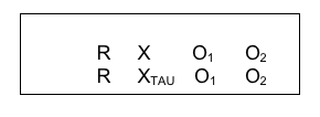
The Variables.
One outcome variable was whether the men entered a treatment program (dichotomous, yes or no). In this example, both the independent (treatment condition) and dependent (treatment entry) variables were categorical in nature; in fact, both were dichotomous categorical variables. Another way of describing this study in terms of the sample is as a 2 X 2 design (2 groups on each variable). For this reason, chi-square analysis was performed on the data.
The Null Hypothesis.
The research question asked was if there existed a significant difference between the outcomes (proportion entering treatment) for men who received the innovative intervention compared to men who received only treatment as usual. In statistics logic, the investigators were testing the null hypothesis that the difference between the two groups of men was zero.
H0: There exists no statistically significant difference in proportion of men entering treatment between those who do and do not receive the innovative intervention.
If the results of analysis led the investigators to reject the null hypothesis, it means they could be reasonably confident that there existed a meaningful difference in treatment entry related to whether the men received the innovative intervention or the treatment-as-usual condition. If the results led the investigators to fail to reject the null hypothesis, they could only say that they did not detect a significant difference.
The Statistical Analysis Approach.
Since both variables were categorical in nature, chi-square analysis was appropriate.
The Analysis Results and Interpretation.
The investigators reported that a total of 56 men participated in the study, with equal groups of 28 randomly assigned to each of the intervention conditions. The authors described the results of their chi-square analysis for entering a treatment program within one week after the intervention as the innovative intervention group having significantly higher treatment program participation than the treatment-as-usual group (75% vs 10.7%), whereχ2(56) = 21.073, p < 0.001 (Danaee-far, Maarefvand, & Rafiey, 2016, p. 1866). Furthermore, they also reported that the rate of retention in treatment at three months follow-up was greater for the innovative intervention group compared to the treatment-as-usual comparison group (60.7% vs. 14.3%) where χ2(56) = 12.876, p < 0.001 (Danaee-far, Maarefvand, & Rafiey, 2016, p. 1866). The authors concluded that the brief social work intervention contributes to treatment participation and retention compared to the usual consulting services for men who use methamphetamines.

Logistic regression.
You now know how investigators might analyze intervention or evaluation data where both the independent and dependent variables are categorical in nature (chi-square). You have ways of analyzing data where the independent variable is categorical and the dependent variable is numeric/continuous/interval (t-test and Anova). You even know what to do when both variables are numeric (continuous) in nature: that is when correlation analysis is often helpful.
What is worth mentioning is the remaining possibility: the dependent variable is categorical and the independent variable is numeric/continuous/interval. In this case, a different approach to analysis is adopted, on the spectrum of what are called regression analyses. These operate from a different set of assumptions and have capabilities that differ somewhat from the parametric analyses we have studied in our two-course sequence. They are based on linear algebra rather than differences in means and variance.
Without going into a great deal of detail, the test that might be used in this case—as long as the dependent variable is a dichotomous (2-category) categorical variable—would be what is called logistic regression. An example might be the outcome (dependent) variable is treatment completion vs drop-out and the independent variable is a numeric variable like age or a score on symptom severity or distance from home to the intervention location. A real-world example comes from the Safe At Home data where treatment completion (or dropout) was related to the number of weeks between the intimate partner violence incident and intake to batterer treatment. While we are not studying this regression approach in detail, it is important to recognize that this analysis approach might be applied to the special case where independent variables are numeric and dependent variables are both categorical and dichotomous in nature.
Stop and Think
 Take a moment to complete the following activity.
Chapter Summary
In this chapter you revisited topics related to univariate analysis, this time in relation to intervention and evaluation research questions and study designs: frequency and proportion data for categorical variables, as well as central tendency and distribution analyses for numeric/continuous variables. You also revisited topics related to bivariate analysis: single sample and independent samples t-tests, analysis of variance, and chi-square analysis. You were briefly introduced to logistic regression and reminded that non-parametric approaches might be preferable to parametric approaches for analyzing small-sample data sets. One important data analysis approach remains to be explored: what to do with longitudinal data, such as the pre-/post- comparison situation. This is the topic of the next chapter in this module.
