Module 4 Chapter 2: Paired t-Test

At this point you have developed skills in the analysis of group comparison data. However, because intervention research designs are often longitudinal in nature, it is time to learn about how comparing pre-/post-intervention data collected from the same participants at two different time points requires a different approach to statistical analysis.

In this chapter you learn:

• the importance of repeated measures analysis approaches for longitudinal data;
• steps involved in conducting and interpreting paired-t test analysis (including an Excel exercise).

Pre-/Post-Intervention Comparisons Are Different (Longitudinal Data)

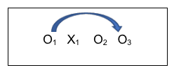
We considered analyses for an intervention research question in Chapter 2 concerning differences in gambling symptoms with and without a novel intervention being delivered—X₁ and wait list no intervention control conditions (Toneatto et al., 2014). The investigators’ design permitted them also to longitudinally examine change in the participants’ gambling symptoms before and after the experimental intervention (X₁). Once the investigators collected the post-intervention outcome data for participants (O₂), they also collected 3-month post-intervention follow-up data (O₃). Let’s look at how they analyzed the data intervention group’s baseline (O₁) and follow-up (O₃) data to see if the observed differences (O₁ to O₂) seemed to hold up over time. Using our study design notation, it looks like this:

Investigators in this situation cannot simply apply the independent samples t-test or the Anova analysis approach as if they had two independent groups to compare because of that longitudinal design. And, this is why…

We already know something about how to statistically compare two groups—but here the investigators did not have two independent groups to compare. Instead, they had the same elements (study participants) being measured twice—before and 3-months after the intervention. In this case, an important assumption in the independent samples t-test and the analysis of variance (Anova) is being violated in the longitudinal data: it is right there in the name of the t-test, “independent samples.” With longitudinal data we no longer have independent groups—by the very nature of having been collected from the same individuals the later round of data is not independent of the first-round data. Participants providing that later round of data are completely dependent on having been the same participants providing the first round of data. This non-independence means that a portion of the variance in the data is due to the individual differences that existed at the first point in time, not due to intervention-caused differences across the two points in time.

Statisticians have developed an elegant solution to this problem in what is called the paired t-test. We use the paired t-test approach in analyzing data where the data involve repeated measurement with the same participants, such as comparing pre- and post-intervention or pre- and follow-up longitudinal data. Paired t-test (and other repeated measure analysis) solutions account for the potential impact of the lack of independence resulting from repeatedly measuring the same individual elements. It is still critically important that the individual pairs of scores be independent of all other pairs of scores (the participants be independent of each other), but it is acceptable that each individual’s longitudinal scores are non-independent at the two points in time—they cannot be since they are produced by the same person. The solution to this problem when comparing two points in time (pre- and post- or pre- and follow-up, for example) is to use a paired t-test instead of an independent samples t-test. In the case of more than two time points being compared, there is an analogous repeated measures analysis of variance, rmanova, to replace the one-way analysis of variance we previously learned—for example, a single analysis that included all three time points, O₁, O₂, and O₃ all together (which is preferable as a means of avoiding a Type II error since it is one less analysis to risk making the wrong decision).

Re-Visiting the Gambling Study Example.

Let’s continue to work the example from the problem gambling study (Toneatto et al., 2014) to examine change in the participants’ gambling symptoms before and at follow-up 3 months after intervention.

The Variables. In this example, the observation (O₁ and O₃) data reflect the problem gambling symptoms variable (DSM symptoms); the example also works for the variable called gambling urges. In this case, the follow-up means were expected to be different from the pre-intervention (baseline) means in the intervention group. As a reminder, both gambling-related variables are numeric in nature, with the scale on each showing that a higher score means a more serious gambling problem. The two points in time represent a dichotomous categorical variable.

The Null Hypothesis (H₀).The primary research question being asked in this analysis is if there exists a significant difference between the pre- and follow-up gambling variable means for the group receiving the experimental intervention (X₁)—is the difference between pre- and follow-up meaningfully different from zero (no difference)? In statistics logic, the investigators were testing the null hypothesis that the difference between the two points in time was zero.

H₀: No difference exists between the pre- and follow-up intervention means.

If the results of analysis lead the investigators to reject the null hypothesis, it means they can be reasonably confident that there is a meaningful difference between the pre- and follow-up means (the difference is NOT zero). If the analysis leads the investigators to fail to reject the null hypothesis, it means that no difference was detected (but they cannot conclude that no difference exists). The investigators are hoping to reject this null hypothesis for the intervention group with both the DSM symptoms and the gambling urge outcome variables.

The Statistical Analysis Approach.

Since the data being compared at exactly two points in time is paired (non-independent), the paired t-test analysis is appropriate. With the exception of this aspect of (non)independence in paired, longitudinal data, the underlying assumptions for this type of analysis are exactly the same as what you learned in our prior course and previously reviewed for the independent samples t-test:

• Type of (Outcome) Variable: The scale of measurement for the dependent variable is continuous (interval).
• Normal Distribution: The dependent variable is normally distributed in the population, or a sufficiently large sample size was drawn to allow approximation of the normal distribution. Note: the “rule of thumb” is that neither group should be smaller than 6, and ideally has more.
• Independent Observations: Individuals within each sample and between the two groups are independent of each other—random selection indicates that the chances of any one “unit” being sampled are independent of the chances for any other being sampled.
• Homogeneity of Variance: Variance is the same for the two groups, as indicated by equal standard deviations in the two samples.

The paired t-test analysis, like the independent samples t-test, involves dividing a difference score by an estimate of variance. The major difference lies in how the difference scores and the variance estimate (square of standard deviation) are handled:

1. calculate the difference score for each individual participant (score_{time 2}– score_{time 1}) and making certain that you preserve the “sign” of each difference as being a positive or negative value;
2. compute the “difference” mean by adding together the individual participants’ difference scores and dividing by the number of participants (this is why it is important to preserve the “sign” for each difference score because you may need to add in some negative numbers along with some positive numbers)—this value will be used as the numerator in your calculation of the t-value;
3. for the denominator in your calculation of the t-value, begin by calculating the square of each difference score from step 1, then add these squared differences together (this will be a sum of squares)—it would be written as ∑(difference²);
4. then calculate the sum of the difference scores, square this value, and divide by the sample size, N—it would be written as (∑difference)²/N–notice the difference where the symbol for squaring is located inside the parenthesis and outside the parenthesis;
5. multiply the sample size minus 1 by the sample size—it would be written as (N-1)*(N);
6. compute the t-value denominator as the square root of [(step 3 minus step 4) divided by step 5];
7. compute the t-value as the numerator from step 2 divided by the denominator from step 6;
8. compare the computed t-value with the criterion value using the degrees of freedom for the total N-1 (where N is the total number of participants) and the α<.05 criterion.

The Analysis Results and Interpretation.

The investigators in the problem gambling study (Toneatto et al., 2014) observed a statistically significant difference in pre-/follow-up outcome variables for the experimental intervention group (X₁). Furthermore, the difference was in the desired direction: the follow-up mean scores were lower 3 months following the intervention than at baseline (pre-intervention), indicating less severe gambling symptoms (see Table 1).

Table 1. Outcome measures at 3-months post-intervention compared to pre-intervention baseline (adapted from Toneatto et al, 2014).

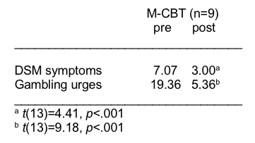
For both outcome measures reported here, the differences between the group means were statistically significant. Thus, the investigators rejected the null hypothesis of no difference (that the difference was zero) and concluded that intervention effects persisted at 3-month follow-up. They believe that mindfulness enhancement of cognitive behavioral therapy for problem gambling warrants further, more systematic research attention. One caution about over-interpreting these results is that intervention of any type is usually preferable to no treatment; future research should compare the mindfulness enhancement to the treatment-as-usual condition or the cognitive behavioral therapy alone.

Stop and Think

Chapter Summary

In this chapter you learned a new statistical approach to bivariate analysis of quantitative data. The paired-t test is one example of repeated measures analysis that is appropriate when the data being compared are not independent because they are from the same individuals at two points in time. You learned why this is important (the estimate of variance needs to be adjusted for this non-independence) and you learned how to engage in this type of analysis. You now know how investigators and evaluators might work with data from most types of intervention and evaluation study designs. What remains is understanding how to work with data generated from single-system design studies. That is the topic of the final chapter in this module.