SWK 3401.3-5.1 Summing Scores

Introduction

The purpose of this activity is to learn how to create a new variable in Excel out of the sum or total of the values for other variables. The example in your coursebook was a hypothetical survey where participants rated on a scale of 1 to 5 their level of agreement with a set of 4 statements. In addition to knowing each individual participant’s answers to these 4 questions, we also want to know their 1 single total score on the scale that combines these 4 items. In this activity, you will create a single, new interval variable by adding up (summing) the 4 ordinal variable scores each participant provided. You could do this simple addition by hand for each person in the survey study, but the chances of making errors is high and the computer is so much faster at it. Let’s make the computer do the work for us.

Instructions

1. Open the Excel data file called: research course survey summing scores example start
2. In your head, or using a calculator, add up the 4 scores that our first student provided (IDnum=1).                       Did you get 14?
3. Instead of doing this calculation 24 more times for the rest of the classmates, make Excel do the work. First, let’s name the new variable in the cell F1. A good suggested name is scale_score. (Remember, you can drag the line between F and G to the right a bit if you are concerned about the column being too narrow for the name.)
4. Next, click on the cell F2. This is where the sum for the person #1 scale score will go. Nothing seems to have happened, and that’s okay. Excel is remembering this as the cell you are interested in.
5. Now click on the down arrow in the upper right corner menu item where you see ∑AutoSum. (The symbol ∑ means “calculate the sum”.) You should see that Excel did you the favor of inserting a function formula that it thinks you want. Excel automatically put in =SUM(A2:E2). This formula shorthand says to Excel: in this cell, F2, I want you to compute the sum of the numbers in cells A2, B2, C2, D2, and E2. (Excel does not like the symbol “-” for to/through in a range, it uses the symbol “:” with a range instead.)
6. Uh, oh. We did not really want this, did we? We did not want to add the person’s id number into the total. To fix this, we can click on that formula that Excel put into the cell for us and simply overwrite the letter A with the letter B. Now we are telling Excel to compute the total of the cells B2 to E2.                                                The answer should appear as 14.
   • Another option: We could just enter in the formula ourselves as =SUM(B2:E2) instead of having to edit the version that Excel did for us. Sometimes it is hard to remember the exact syntax of a command for Excel. A helpful tip is to go to the tab on the top menu bar that says “Formulas” and when you click on it, the first option is fx Insert Function. Then, in the drop-down menu, select SUM and at the bottom of the box it shows you just what will happen with that function (adds all the numbers in a range of cells). To find out how to hand enter the function, click on the “help with this function” option and it takes you to a support page that shows you to type in =SUM(A2:A10) to get the sum of values in cells A2 to A10 (as an example). Or you can watch the short video. The temptation is to put in the range as A2 – A10 but remember: Excel doesn’t recognize the – symbol; you have to use : instead.
7. It would be tedious to have to redo steps 5 and 6 an additional 24 more times. Excel gives us the gift of a smart shortcut. Click on the cell F2 and a copy command (on a PC, it is Ctrl C); or, you can click on the cell F2 and right click for the menu that has “copy” as an option. This should put a box around the cell with moving dashed lines.
8. Then, click on the next cell down, F3, and drag to highlight all of the cells down to F26, and paste. You might expect that every one of those cells would end up with the score 14, right? But Excel is smarter than that—click on the cell F6 for example and in the large white box at the top of your screen you will see the formula used for that cell: =SUM(B6:E6). Excel knew to change the range of cells in the formula!
9. Just to be sure, try adding up the scores on the 4 items in the 6th row, for person #5. Did you get the same answer as Excel (9)? (Remember, we do not want to accidentally add in the ID number.)
10. Your finished file should look like this:
    
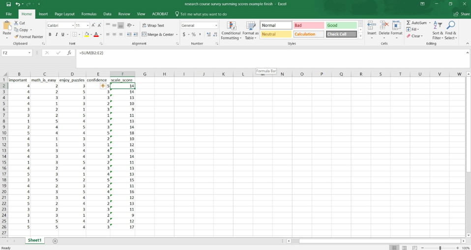
11. You will want to save your file because we are going to work with it again in a future activity—give it a meaningful name so that you can find it again next time. (No big deal if it gets lost, though.)
12. Congratulations! If you work looks like the file in item #10, you successfully completed this activity and have computed the new variable.