SWK 3402.3-4.3 Exercise Testing Randomization with Independent Samples t-Test Analysis

INTRODUCTION

The purpose of this activity is to learn how investigators might check the success of their randomization efforts with regard to a scale (continuous) variable. This time we are looking at an intervention where investigators were going to measure the impact of a high school dating violence prevention lecture on the students’ attitudes toward hitting in a dating relationship. The study design was a pre-/post- intervention survey involving N=757 students. For the purposes of this example we will pretend that students were randomly assigned to two conditions: receiving the intervention (n=247) and not receiving the intervention (n=510).  In reality, the original variable “present both days” (since absenteeism was high in this school system) has been transformed for our example into a hypothetical randomization condition variable—the group receiving the intervention or the no-intervention control group.

The investigators used an instrument constructed for this project where 743 of the N=757 students responded to five scenarios where the male partner in a dating relationship hit the female partner. Students rated from 1 to 5 how much the female partner deserved to be hit: 1=deserve it, 3=might deserve it, 5=does not deserve it. The scenarios involved hitting because:

• she yelled at him,
• she won’t listen to him,
• she talks to another boy,
• she hits him,
• she refuses to have sex with him, and
• she insults him in front of his friends.

A composite “deserving” score was computed by adding together each student’s ratings for these six items. The investigators  hope that the two randomly assigned groups (intervention and no-intervention control) are equally distributed in terms of their composite “deserving” scores at the outset, before the intervention is delivered (the “pre” data). Then, any differences between the two groups detected in the post-intervention data might be attributed to the intervention. The proper statistical analysis for testing the difference in means between two groups is the independent samples t-test.

INSTRUCTIONS

1. Open the file called “randomization t test” in Excel.
2. The variables of importance to this analysis are the last two in the list: condition (intervention or control group) and deserves (the composite sum of ratings for the six items at pre-intervention testing).
3. Given the large number of steps we had to take in computing the chi-square analysis, you might expect the t-test to be more complicated than it actually is. Fortunately, there is only one main task involved in the calculation process! Unfortunately, our data file is not configured the way that Excel needs it configured to execute this analysis. We need to do a little reconfiguration work on the data file up front. So, like the chi-square analysis, we are going to spend some time up front before we can do the computation of interest. The reconfiguration goal is to have the values on our scale (continuous) variable called “deserves” in one cluster for the students who were hypothetically randomized to the intervention condition (“condition” variable is coded as 1) and in a separate cluster for students randomly assigned to the control condition (“condition” variable is coded as 2).
4. This reconfiguration task is most easily accomplished by first sorting the cases on the condition variable so that the “1s” and “2s” are separated into two clusters. This process begins with selecting all of the data in the file (select all in PCs is “Control A” or you can simply click and drag to include all of the data). Otherwise, the sort only happens in the one column and the other data do not rearrange with it—this is a major flaw in Excel to be aware of!
5. Then, in the top menu bar, select the “data” tab. In the next level menu, select the “Sort” tab. This should open a dialogue box where you designate sorting by the “grouping” variable in our analysis—condition. We want the data sorted on cell values (the entry 1s and 2s) and the order does not really matter, smallest to largest is fine. When you click on “ok” you will see that your data have been reorganized for you. The intervention group (condition=1) is in rows 2 through 248, and the control group (condition=2) is in rows 249 through 758.
6. Now, you need to select and copy all the values in the “deserves” column where the “condition” value is a 1. This is cells P2:P248. Then paste it into an empty column—R would be a good choice, starting with R2. Then, place a label at the top of this new column—intervention is a decent choice for cell R1.
7. Repeat this process with all the “deserves” values from P249:P758 to pick up values where the “condition” value is 2. Paste it into another empty column (S is a good choice) starting with row 2 (S2) and label this column something like “control” in cell S1. Completing these steps means you have now created 2 new data columns by copying/pasting the data of interest on one variable (deserves) for two groups (condition=1 and condition=2) into two new “variables” in Excel logic—these are not really “variables” the way we have learned about them, they are two categories of data separated on one dichotomous variable. But this is the logic/language that Excel has adopted, so we’ll have to live with it and not let it confuse us.
8. Now that the data are properly configured, the next step is to click on “data” tab in the menu bar and double-click on “data analysis” in the upper right corner of the top menu bar. This opens the menu of statistical analyses available—the event you have been looking forward to completing!
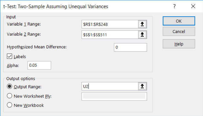
9. Scroll down the list and select the one called t-test: two-sample assuming unequal variances. When you click “ok” you see a dialogue box with information to be filled in about your analysis. The top two blanks are for designating where your input data are located—for “variable 1” (the deserves values for the intervention group) and variable 2 (the deserves values for the control group). But, since we want to have the column labels included (see selecting “labels” in step 7 below), we actually use the range for the first group (called “variable 1” in Excel) as R1:R248 and the range for the second group (called “variable 2” in Excel) as S1:S511. The actual syntax for these two “variables” is:    $R$1:$R$248   and  $S$1:$S$511   in the two blanks.
10. Filling in the remaining information for the dialogue box, we set the hypothesized mean difference to match our null hypothesis: 0. And we want to select labels (what we put into cells R1 and S1). The alpha default in Excel is what we would have chosen: α=.05 and we want it to present the results in a section of our worksheet—maybe have it start in cell U2. It should look like this:
    
    
11. When you click on “ok” results of the analysis should appear in your open worksheet.
12. Let’s assess the results of this independent samples t-test. The mean deserve score for the intervention group (M=27.96 with rounding) is higher than the mean for the control group (M=26.28)—the intervention group was answering more as we would like them to (hitting not being deserved). But this difference may or may not be statistically significant. The t-statistic computed for the 623 degrees of freedom in our data was t(623)=5.76, and the critical value for a two-tailed test of the t-statistic is 1.96 at this many degrees of freedom. Unfortunately, we reject the null hypothesis of no difference because the t-statistic is greater than the critical value. This is bad news for the investigators who were hoping for a successful (hypothetical) randomization of the students—here, the intervention group (hypothetically) started out significantly better off than the control group, so differences after the intervention cannot be attributed to the intervention alone.
13. Another way of looking at this situation is that we reject the null hypothesis of no difference between the two condition groups because the p-value of 1.3E-08 is less than our .05 criterion. As a reminder, in scientific notation, the E-08 means there are 8 decimal places to the left of where it appears in the base number. Here, our p-value is .000000013.
14. Feel free to compare your output to the output in the file named “randomization t test finish” and if your results are similar and you drew the same conclusions, you have successfully completed this activity!