SWK 3402.3-4.2 Exercise Testing Randomization with Chi-Square Analysis

INTRODUCTION

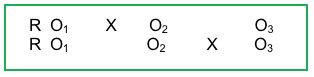
The purpose of this activity is to learn how investigators might check the success of their randomization efforts with regard to a nominal (categorical) variable. This example involves having 2 treatment conditions (an experimental group, coded as 1, and a delayed treatment control group, coded as 2) where participants were randomly assigned to a condition (group) as they enrolled in the study. The investigators determined that they could provide immediate service to about 1/3 of the study participants and then to the remaining 2/3 as a delayed treatment condition. The study design would look like this:

The investigators are concerned that there may exist an influence of gender on the outcomes and are hoping that men and women were assigned to the two groups in equal proportions (gender is based on self-identified categories, and only two categories appeared in the data, coded as 1=man, 2=woman). Because both of our variables (group, gender) are nominal/categorical variables, the test to use is the chi-square (χ²) analysis.

Let’s begin by stating the null hypothesis for this analysis (H₀).

H₀: No difference exists in the proportion of men and women assigned to the experimental and control groups.

Now, let’s test this null hypothesis. Remember: the investigators are hoping NOT to reject this null hypothesis, since they hope the groups might be equivalent (no difference) in this test of our randomization success. (This is different from when investigators test the hypotheses related to their research questions—there, they WOULD hope to reject the null hypothesis of no difference between the experimental and control treatment conditions.)

INSTRUCTIONS

1. Open the data file called “randomization test chi square” in Excel. Most of our work will revolve around setting up to conduct the analysis—the actual analysis itself is quick.
2. First, let’s review how to find out how many men and women are in the total sample, and how many individuals were randomized to each of the two conditions. The command to use is the =COUNTIF command. So, ask Excel to count how many individuals were coded as “1” (men) for this variable—it would be =COUNTIF(C2:C179,1) because we want it to count all of the “1s” in the cells numbered C2 to C179. To begin creating a contingency table, place this command in the cell numbered J4. It would help to have the label “totals” typed into the cell above (in J3).
3. Then, repeat this action for the women in cell J5—it would be =COUNTIF(C2:C179,2) because we want it to count all of the “2s” in the cells numbered C2 to C179. It helps to type in labels for these categories, perhaps in cells G4 (men) and G5 (women).
4. Now repeat these actions for the next variable which is the group to which each participant was assigned—in cells H6 and I6 (column capital “I” and row 6, not 16). It would be =COUNTIF(B2:B179,1) and =COUNTIF(B2:B179,2) and you will want to type in labels, experimental and control, in cells H3 and I3. Also, the label “totals” could go in the cell G6.
5. It also helps to know the total number of cases in the sample. That is easily done with the command =COUNT(B2:B179) in cell J6.
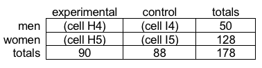
6. The next step is to test the null hypothesis that the proportions of men and women in the two groups are no different. Our contingency table, copied into cells G3 to J6 at this point looks like this:
   
7. To completely fill in this contingency table we need to first count how many men were in the experimental group (cell H4). The easiest way to accomplish this task is to sort the data from low to high on the variable called gender, then count the number of experimental cases (coded as 1 on the group variable) just those in the range of cells where “1” is entered for gender (1 for men). The first part of this step is accomplished by highlighting all the data from cell A2 to C179, selecting “data” in the top tool bar, and “sort” in the next tool menu down. You will want to select “gender” as the option in the “sort by” box, and the defaults cell values and smallest to largest order are fine choices.
8. The men appear in rows 2 through 51. Thus, we want to use this information in our COUNTIF command. In the proper cell of our contingency table for men in the experimental group (cell H4) enter the command =COUNTIF(B2:B51,1) to find how many of the men (rows 2 through 51) were in the group coded as 1 (the B column).
9. Then we need to count how many men were in the control group. So, in the proper cell of the contingency table for men in the control group (I4 is the capital letter “I” and number 4, not 14) should have the following command entered: =COUNTIF(B2:B51,2).
10. Next we need to count how many women were in the experimental group. Women appear in rows 52 to 179. So, in the cell for women in experimental group (cell H5) we would enter the command =COUNTIF(B52:B179,1).
11. And we need to count how many women were in the control group. In the final empty cell, I5, enter the command =COUNTIF(B52:B179,2).
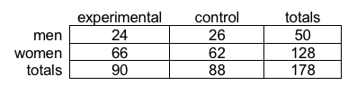
12. At this point, our contingency table looks like this:
    
13. Sigh. We still have not gotten to the point of calculating the chi-square (χ2) statistic for these data. That is what comes next. Excel needs to compute for us the Expected values for each cell in our contingency table—we currently have only the Observed values. The simplest next step is to copy and paste our current Observed values contingency table into a new spot, then delete the observed value cells and get them refilled with the Expected values. The copy operation includes cells G3 to J6; paste the copied table into cells G9 to J12 for the next steps to make the most sense to you.
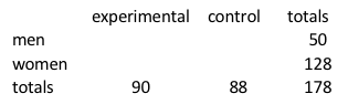
14. Delete the data currently in the observed data cells, leaving only the 178 in the final total. Then, type in the 4 totals (not the formulas) from the observed values table.Your table should look like this:
    
    
15. Next, you are going to ask Excel to compute the proportions for each empty cell, multiplying the associated column and row totals and dividing by the overall total (178).
    The Expected values formula in general will be the (row total * column total)/ total N (where * means multiply).
    • in cell H10 (experimental, men) the syntax is=(H12*J10)/J12, and the expected value is 25.28 (with rounding).
    • in cell I10 (control, men) the syntax is =(I12*J10)/J12, and the expected value is 24.72 (with rounding)—note the use of the capital “I” not to be confused with the digit “1”.
    • in cell H11 (experimental, women) the syntax is =(H12*J11)/J12, the expected value is 64.72 (with rounding).
    • in cell I11 (control, women) the syntax is =(I12*J11)/J12, and the expected value is 63.28 (with rounding)—again, take care not to confuse the letter “I” with the digit “1”.

    The Expected values table should now look like this (before rounding):
    
    

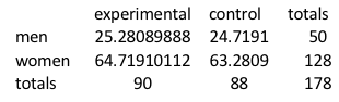
16. Now, we are ready to ask Excel to calculate the probability that the difference between the Observed and Expected values (proportions) is zero—our null hypothesis. Remember that the formula for computing the χ²test statistic is:
    χ²=∑ (O_r,c– E_r,c)²/ E_r,cIn plain English, this means we are going to do the following steps:
    
    • For each cell, subtract the expected (E) value from the observed (O) value–that is the (O – E) for each cell’s row/column location
    • Compute the square of that result
    • Divide that squared result by the expected (E) value for that cell
    • Add up (sum) the results for all four of the newly computed cells together (∑).

    Remember also that Excel needs syntax placed in (parentheses) to tell it the order of the operations—if we said O-E2/E, it would subtract E2/E from O and that would be a very different answer.

    Remember that the sign for squaring a value in Excel is a “^” symbol (the carrot top symbol over the number 6 on a keyboard).

    Here is the way we are going to make all of this happen using Excel:
    

    • In cell H15, the syntax is: =((H4-H10)^2)/H10 [the result is 0.065 with rounding]
    • In cell H16, the syntax is: =((H5-H11)^2)/H11 [the result is 0.025 with rounding]
    • In cell I15, the syntax is:   =((I4-I10)^2)/I10  [the result is 0.066 with rounding]
    • In cell I16, the syntax is: =((I5-I11)^2)/I11  [the result is 0.026 with rounding]
    • In a new, empty cell (try H18), we find the sum total of these four values by entering a sum command =SUM(H15:I16) which is 0.183 with rounding.
17. Finally, we can use a chi-square distribution table with the degrees of freedom for this test to find the criterion value for comparison of our computed χ²test statistic. Our degrees of freedom are computed as: (number of rows – 1) * (number of columns-1). In our case, we have 2 rows and 2 columns, so our degrees of freedom are (2-1) * (2-1) which is 1*1, and the result is df=1 for our analysis.
18. The comparison statistic comes from Excel if you place the following syntax into any empty cell (try H19): =CHISQ.INV.RT(0.05,df), where df is filled in for our degrees of freedom. In our case, the critical value syntax is: =CHISQ.INV.RT(0.05,1) and the result is 3.841 (with rounding). Since our χ² test statistic value of 0.183 is smaller than our criterion value of 3.841, we fail to reject the null hypothesis. Which, in this case, is a big relief since we were hoping NOT to find a difference in the proportion of men/women in our experimental/control groups.
19. In case you wish (or need) to report the test’s corresponding p-value, this is done with Excel by using the syntax =CHISQ.TEST(observed cell range, expected cell range). So, in our example, the syntax is: =CHISQ.TEST(H4:I5,H10:I11), and when this is placed in any empty cell (like H20) the result is p=0.669. Again, we fail to reject the null hypothesis because the p-value for our computed χ² is greater than our α criterion of .05.
20. Whew! That was a lot of work, but we found the answer to our question. Feel free to compare your working results with those presented in the file named “randomization test chi square finish”. If you obtained similar results and drew the same conclusions, you have successfully completed this learning activity. Congratulations!