SWK 3401.4-2.4 Computing Descriptive Statistics (Mean, Median, Standard Deviation)

Introduction

The purpose of this activity is to learn how to use Excel to compute multiple (univariate) descriptive statistics for a set of values about a variable—all in one step. We will use the data presented in the coursebook about student absenteeism for this exercise, finding the mean (average) number of days that students in this class were absent.

Instructions

1. Open the file called student absenteeism start.xlsx
2. This time you want to use the Data Analysis functions that open only after the Data Analysis Toolpack is downloaded and you have selected the Data tab in the top menu bar.
3. Click on the Data tab, then double click on Data Analysis (all the way on the right). A menu of statistical analysis tools opens for you.
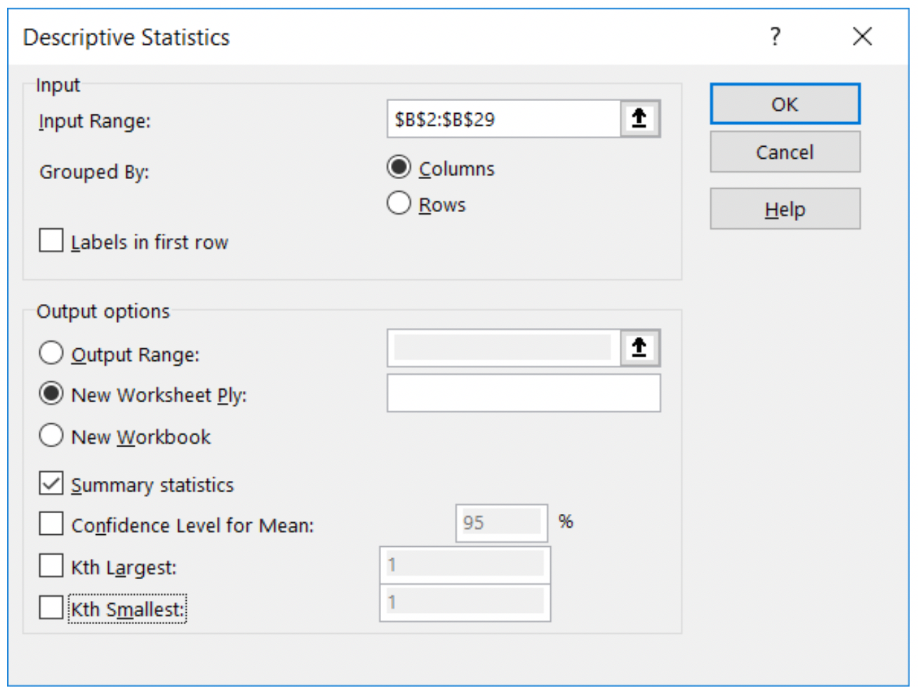
4. Select the option called Descriptive Statistics and click OK.
5. Now Excel wants some more information about what you want it to do. The input range refers to the values for which you are seeking the descriptive statistics. In our case, this is B2:B29. Excel will want this to read as: $B$2:$B$29 and should do this adjustment for you (if it doesn’t, type it in that way—the $ signs make it clear to Excel that these are cell addresses).
6. In the next area, select New Worksheet Ply and leave the space blank. (This will put the answers on a new sheet so you don’t clutter up your data file.)
7. Select Summary statistics (this will be the mean, median, mode, standard deviation, sample variance, range, minimum, maximum, sum, count) If your box looks like this, then click on OK.
   
8. Excel takes you to a new sheet, called Sheet 2 (see the bottom of your screen; Sheet 1 is your data sheet that you were looking at before).
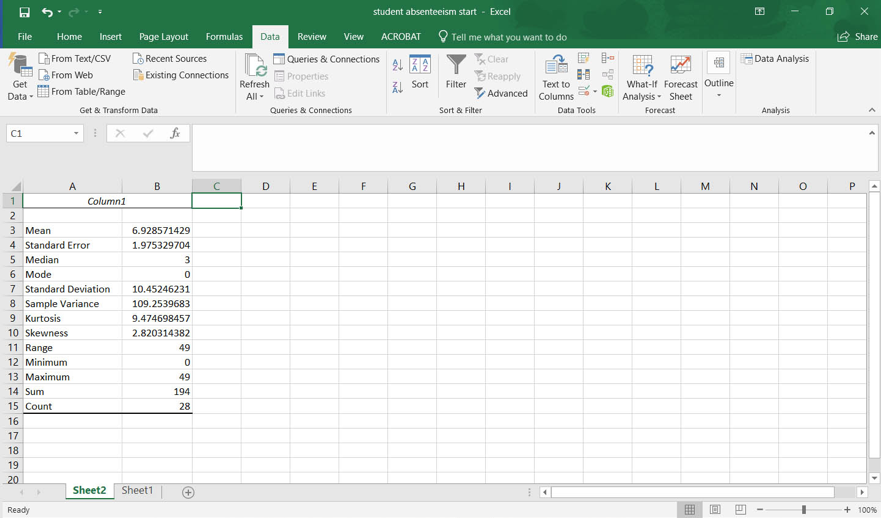
9. After clicking on the line between column A and column B and dragging it to the right (widening column A; you can widen column B also if you like), your output should look like this:
   
10. Now let’s spend a few minutes interpreting the information Excel provided to us.
    • The mean number of days absent was 6.93, as we found in our earlier exercise.
    • The median number of days absent was 3 (the 50thpercentile where half of the values were less, and half were more).
    • The mode was 0 (the most common value).
    • The standard deviation was 10.45 days absent.
    • The sample variance was 109.25. (If we square the standard deviation, we get this number: (10.45)2=10.45 x 10.45=109.25).
    • The fewest number of days absent was 0 and greatest number of days absent was 49.
    • The total number of absent days for the whole class combined was 194 days.
    • There were 28 children for whom we had data.
    • If you wanted to check the mean, you may recall we divided 194 days by 29 children to find a mean of 6.93.
11. If your results look like this, then you have successfully completed this activity! (We will learn about skewness and kurtosis later, when we learn about normal distribution.)