SWK 3402.3-4.4 Exercise Testing Randomization with Analysis of Variance (Anova)
INTRODUCTION
The purpose of this activity is to learn how investigators might check the success of their randomization efforts with regard to a scale (continuous) variable. In this exercise you will be working with a portion of data from a randomized control trial (RCT) of a screening and brief intervention conducted with women scheduled for release from jail within two weeks. The full study followed the women during early reentry (Begun, Rose, LeBel, 2011). The women were randomly assigned to the experimental intervention or the treatment-as-usual (TAU) condition using Uno game cards that each woman drew at the time of screening. The investigators were hoping that their randomization efforts resulted in two groups where the Alcohol (and other drug) Use Disorder Test (AUDIT-12) scores were comparable at the start, before the intervention was delivered. Thus, any differences observed at the end could be attributed to the intervention and not to initial differences on this measure. All of the women scored in the “positive” screening range on the AUDIT-12 screening measure—this was an inclusion criterion. In the actual study, the groups were unequal in size, but for this exercise each group has n=236 participants because Excel cannot do analysis of variance (Anova) tests with groups of unequal size. Statistical programs like SPSS and Stata can make the necessary adjustments.
Let’s start by specifying the null hypothesis (H0) for our analysis—the hypothesis that we actually hope NOT to reject because we hope the two groups might be equal.
H0: There is no difference in mean audit total scores between the pre-intervention experimental and treatment-as-usual (TAU) control groups.
NOTE: Because there are only two groups, we could use an independent samples t-test for this analysis and would obtain the same results (the F-statistic is the square of the t-statistic)–you will see this in the later steps of this exercise. For now, remember that if there had been 3 or more groups, we would have to use analysis of variance (Anova) to compare group means.
INSTRUCTIONS
1. Open the file called “randomization anova women in jail.xlsx” in Excel.
2. The AUDIT-12 variable is called “auditot” (for the total score) in this data set, and the variable concerning which group women were randomized to is called “random” where 1=experimental and 2=TAU group.
3. Once again, we are faced with the problem that our data set is not configured the way that Excel needs it to be configured to conduct this analysis. We need to do the same thing that we did for the independent samples t-test: create 2 new columns of data to be compared. So, the first step is to sort the data on the grouping variable (random) to pick up the values on our scale (continuous) variable sorted into two new columns
4. First, select all the data (cells A2 to C473), select “data” from the top menu bar, and select “sort” in that drop-down menu. Note: if you select the cells A1 to C473 you can check “my data has labels” if you like. The sort by blank should be filled in with the variable “random” and the rest of the defaults should be fine. You should see the split happening at row number 237—everyone above that row is coded as “1” and everyone below that row is coded as “2.”
5. Next, select the auditot values for the participants who were randomized into group 1 (experimental)—the data in cells C2 to C237. Copy and paste these values into a new column—start with F2 perhaps. Then type in a label in F1, “experimental” is a good choice of label. You will see that the auditot scores for the experimental group appear in cells F2 to F237.
6. Repeat this step with the auditot scores for participants where were randomized into the TAU group (coded “2” in the random variable). These values are in cells C238 to C473. Copy and paste these scores into a new empty column: G would be a good choice. Then, label the top of the column in cell G1—either TAU or control would be good choices for the label. You will see that the auditot scores for the TAU control group appear in cells G2 to G237.
7. Now that you have the data reconfigured for Excel analysis you are ready to request the analysis of variance (Anova) test. Begin by selecting the “data” tab in the top menu bar, then “data analysis.” In the data analysis selection menu, you want the Anova test called single factor—this is what a one-way analysis of variance is called in Excel.
8. To fill in the dialogue box that opens you need to tell Excel the input range of cells for the two groups of auditot data—the data are in cells F2:G237. But, we do wish for the labels to show in our output, so the syntax for the input box will be as follows:
$F$1:$G$237
The data are arranged in columns, so that should be marked.
The box for labels should be checked.
A good place to start the output would be in cell J2 (output range).
9. Once you select “ok” your output should magically appear. Let’s look at what this means. First, we see the two group means appear to be quite similar—in the “Average” column we have M=25.13 for the experimental group and M=25.83 for the TAU control group.
10. Looking in the second box, we see the F-statistic calculated from our data is F=0.575 and that F-statistic has a p-value of 0.45 (with rounding). Excel has told us that the critical value for Fat 1 and 470 degrees of freedom is 3.86, and we continue to rely on the α<.05 decision rule. In other words, we fail to reject the null hypothesis of no difference in Anova scores for our two groups because the F-value of 0.575 is less than the criterion value of 3.86; also, our p-value is greater than .05. Hooray! This is what was hoped for!
11. While the job is done, there is one more demonstration point to explore in these data. Remember that a one-way Anova for 2 groups is the same as (the square of) an independent samples t-test? Here is proof of that point. Since the data are already arranged for us in the two columns, it is a simple task to ask Excel to compute the t-test for us to compare. Go back up to “data” and “data analysis” and this time select the option for t-test: two-sample assuming unequal variances. Fill in the box so it looks like this:
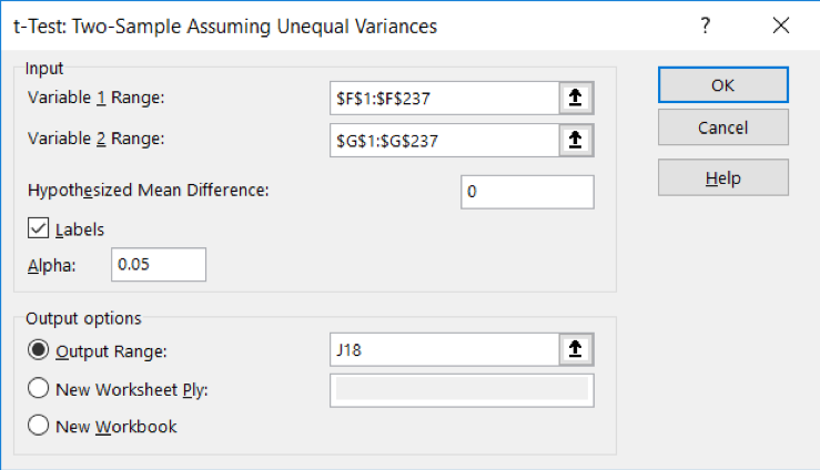
You should see that the means and variances are the same, and the count and observations are the same as in the Anova output. The t-statistic computed for the difference in the two group means is -0.758 which is NOT the same as the F-statistic. But, we said that F is the square of t, so over in cell M26 ask Excel to compute the square of the t value—this can be done one of two ways. You can either use the command =K26*K26 (multiply the value in that cell by itself) or =(K26)^2 which is the command for squaring a value. Now you see the value is 0.575 which was the value we found for F in the Anova test.
Even without comparing the F and t values, we see that we came to the same conclusion: fail to reject the null hypothesis of no difference in the two groups’ means because the critical value for t at 467 degrees of freedom was 1.965 and our observed value of t was less than this critical value; also, the p-value in our test was 0.45 which is greater than our decision rule of α<.05.
12. Feel free to compare your output to the file named “randomization anova women in jail finish”. If you obtained the same results and drew the same conclusions, you have successfully completed this learning activity! Nice job!
Reference
Begun, A.L., Rose, S.J., & LeBel, T.P. (2011). Intervening with women in jail around alcohol and substance abuse during preparation for community reentry. Alcoholism Treatment Quarterly, 29(4), 453-478.
