Module 4 Chapter 4: Principles Underlying Inferential Statistical Analysis
In addition to using inferential statistics to estimate population parameters from sample data, inferential statistics allow investigators to answer questions about relationships that might exist between two or more variables of interest (bivariate analyses). Inferential statistics help test initial hypotheses about “guessed at” relationships between study variables. In other words, investigators infer answers to quantitative research questions about populations from what was observed in sample data. In prior modules, you learned about study design options that maximize the probability of drawing accurate conclusions about the population based on sample data. Now we examine how to use inferential statistics to test bivariate hypotheses. To understand our level of confidence in the conclusions drawn from these statistical analyses, we first need to explore the role played by probability in inferential statistics.
In this chapter, you will learn about:
- probability principles and the role of probability in inferential statistics
- principles of hypothesis testing and the “null” hypothesis
- Type I and Type II error.
Understanding Probability Principles
You think about and calculate probability often during the course of daily living—what are the chances of being late to class if I stop for coffee on the way, of getting a parking ticket if I wait another half hour to fill the meter, of getting sick from eating my lunch without washing my hands first? While we generally guess at these kinds of probability in daily living, statistics offers tools for estimating probabilities of quantitative events. This is often taught in terms of the probability of a coin toss being heads or tails, or the probability of randomly selecting a green M&Ms® candy from a full bag.
Let’s see what happens when we consider the probability of drawing a blue card from a deck of 100 Uno® cards—Uno® game card decks have equal numbers of Blue, Yellow, Red, and Green cards: 25 each (ignoring the un-numbered action and wild cards). In drawing one card from the deck, we have 100 possible outcomes—our draw could be any of the 100 cards. You may intuitively see that we have a 1 in 4 probability of blue being drawn (25%).
The following formula captures the probability of drawing a blue card (Pblue) in this scenario:
Pevent = # of times event is possible / # of total possible
In other words:
Pblue = # of blue cards/# of total possible, or Pblue = 25/100 = ¼ = 0.25 = 25%

It is only slightly more complicated to determine the probability of a blue card being drawn later in the game, when the shuffled deck has been drawn down in play: for example, only 8 cards remain in the draw pile: 3 blue, 2 red, 2 green, and 1 yellow card. Now what is the probability of drawing a blue card? Again, we apply the probability formula, plugging in the different values.
Pevent = # of times event is possible / # of total possible
Pblue = # of blue cards / # of total possible
Pblue = 3/8 = 0.375 = 37.5%
It is up to you to decide if you want to risk the outcome of the game on this chance of drawing a blue card!
Probabilities have at least three interesting characteristics. It is helpful to consider each of these three in a bit more detail.
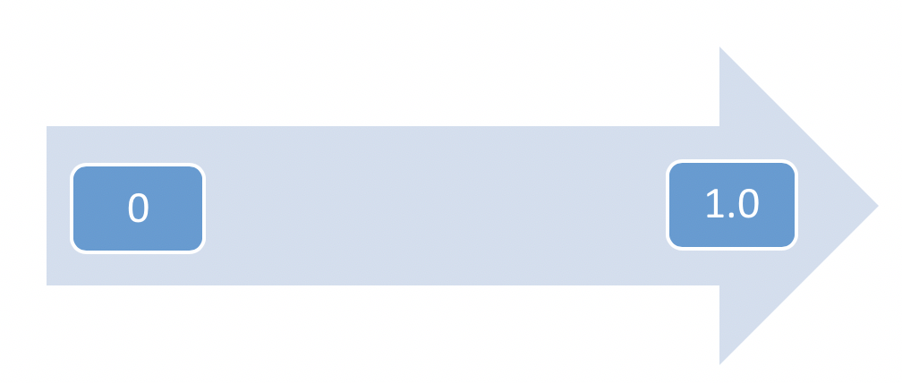
Probabilities exist on a continuum. The continuum of probabilities is from 0 to 1.0—from absolutely no chance to a 100% guarantee.
Probability differs from chance. This rule is at the heart of what is called the gamblers fallacy. Assuming that two possible outcomes have equal chances of happening (heads/tails on a coin, or having a girl versus a boy baby), it is possible to calculate the probability of any particular sequence occurring. Imagine that a couple has 3 daughters and are expecting their 4th child. They want to know whether they can expect the next child to be a boy. The answer is: the chance of having a boy remains the same—whether this is their first baby or their 10th baby. The chance remains 1 in 2, or 50%.
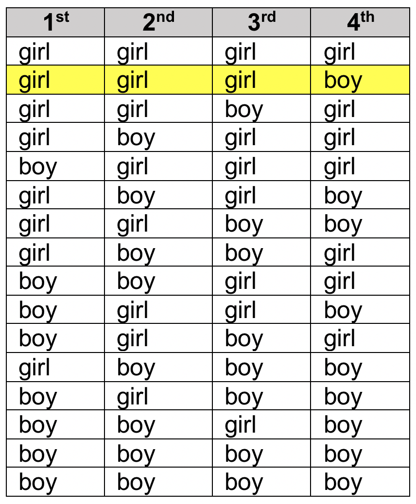
The probability question is a bit different than they expressed, however. They may not really be asking the probability of having a boy, they are actually asking the probability of having a family composition that is girl, girl, girl, boy. In that case, we can multiply the chance of each individual event happening to get the probability of the total combination happening:
1/2 girl x 1/2 girl x 1/2 girl x 1/2 boy
The result is 1 x 1 x 1 x 1 =1 for the numerator, divided by 2 x 2 x 2 x 2 = 16 for the denominator. In other words, the probability of this combination happening in this order of births is 1/16, or 0.625 or 6.25%. Remember there are many other possible combinations that the family could have had if the order does not matter, including no boys, one boy, two boys, three boys, or four boys among the girls, and each possible combination having the same probability of occurring in specified order (1 in 16):
The gambler’s fallacy confuses the chances of the next child being a boy (1 in 2, or 50%) with the probability of a whole sequence/pattern occurring (girl, girl, girl, boy being 1 in 16, or 6.25%).
Remember: this only applies if the chance of the event happening is random—if there is a biological reason why boys are more or less likely than girls, the entire formula for probability will need to be revised. It is called the gambler’s fallacy because people mistakenly bet on certain outcomes, confusing chance with probability. A real-life example presented in an online article about the gambler’s fallacy (www.thecalculatorite.com/articles/finance/the-gamblers-fallacy.php) described a spectacular event that occurred in August of 1913 at a Monte Carlo casino: the roulette wheel turned up the color black 29 times in a row, the combined probability of which was 1 in 136,823,184! The article’s authors stated, “After the wheel came up black the tenth time, patrons began placing ever larger bets on red, on the false logic that black could not possibly come up again.” Obviously, it did, 19 more times. The gamblers’ logic was false because the chances of black coming up was always 18 out of 37 times on this type of roulette wheel (48.6%). Therefore, each of those 29 times had an 18/37 chance of being black, regardless of what happened in prior spins. Do you see how this chance of an event (18/37) differed from the probability of the whole sequence occurring (1 in 136,823,184)?
Inverse probability. When there exist only mutually exclusive events, the probability of a specific event happening and the probability of that specific event NOT happening add up to 1. Thus, the probability that it will happen is the mathematical inverse of the probability that it will not happen. In other words, subtracting the probability that it will happen from 1.0 gives you the probability that it will not happen; and, vice versa, subtracting the probability that it will not happen from 1.0 gives you the probability that it will happen.

As an example, let’s go back to our probability of drawing a blue card from the whittled down play deck with only 8 cards left. We computed the probability of a blue card (Pblue) as being 0.375. Therefore, we can apply knowledge of inverse probability if we want to know the probability of drawing something other than a blue card (Pnotblue is the combined probability of drawing red, green, or yellow):
Pnotblue = 1.0 – Pblue
Pnotblue = 1.0 – 0.375 = 0.625

Take a moment to complete the following activity.
Probability Principles Applied in Statistics
Probability is about the likelihood of an outcome. Remember that with inferential statistics we can never know with 100% certainty that our sample data led us to the correct conclusion about the population. This is where probability comes into play in the process of engaging in inferential statistical analyses. The following scenario helps make the case:
- Imagine you draw a random sample from the population for your study, accurately measure the variable of interest, and compute your sample statistics (for example, the mean and standard deviation for an interval variable).
- Now, imagine that you “put back” those sampled participants and draw a new sample. With random selection, any of the previous participants and all the other possible participants in the population still have an equal chance of being drawn (we learned about this in Module 3, chapter 6 about random sampling).
- You repeat your measurement process and compute your new sample statistics. Because there are different participants this time, and there exists variability between individual participants, your sampling statistics for the different sampling groups will most likely be somewhat different—maybe a little different, maybe a lot different.
Which computed sample value is more “right” in describing the full population? The answer is: neither or both, and there is no way of knowing the population’s true value without measuring the entire population (we learned about this in Module 4, Chapter 3). So, imagine your next step is to keep drawing samples, measuring, and computing the sample statistics for each sample drawn. Eventually, for a variable that is distributed normally in the population-as-a-whole, the sample statistic values that you computed over hundreds of trials (samples) will be approximately normally distributed—you learned about normal distribution in Chapter 4 of this module.
For example, imagine that you were computing the mean on a variable “number of hours each week spent working on issues related to someone’s alcohol misuse” for each sample of social workers drawn 1,000 times—some social workers spent virtually none of their time in this type of activity while other spent almost all their time this way. Your first sample’s mean number of hours was 15, your second sample’s mean was 12, your third sample’s mean was 22, and so on until you have 1,000 mean values for your drawn samples. If this variable is normally distributed across the population of all social workers and you drew each of your samples randomly from the population of social workers, those mean values would come close to looking like a normal “bell” curve. At this point:
- You could compute the mean-of-means for the whole set of 1,000 samples. This sample mean-of-means would be a reasonable estimate for the population mean (population parameter).
- Knowing the mean-of-means value, you could compute the standard deviation for the mean number of hours across your 1,000 samples. The sum of squared distances for each sample’s mean from the mean-of-means divided by 999 would be the variance, and the square root of the variance is the standard deviation (you learned about variance and standard deviation in Chapter 2 of this module).
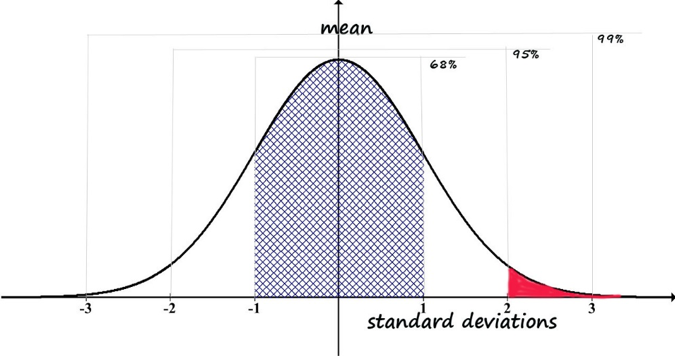
Figure 4-1 is the same normal curve introduced earlier, this time with the notation that the x-axis (horizontal) represents the computed values for the 1,000 sample statistics, and the y-axis (vertical) represents the frequency each computed value for the sample statistic was the result. Note that our unit of analysis is no longer each individual social worker’s hours—that was the unit of analysis in each of our 1,000 samples. Now the unit of analysis is the mean for each of those 1,000 samples.
Figure 4-1. Normal distribution around the mean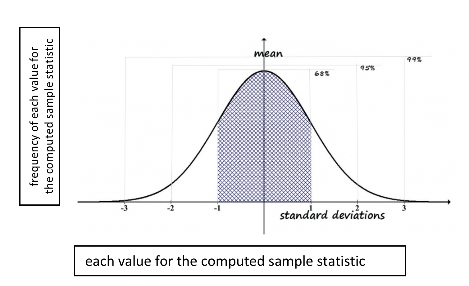
In reality, no investigator would set out to repeat a research study this many times. However, the investigator who completed the study the first time wants to know: is my sample statistic falling within the 95% range in relation to the true population mean, or does it lie in one of the two tails: the 2.5% below or 2.5% above two standard deviations away, adding up to the remaining 5%? This should sound familiar: it represents the 95% confidence interval (CI) for the sample statistic!
Using what we learned about the inverse probability relationship, selecting a 95% confidence level means accepting a 5% error rate (100% – 95% = 5%): or, in decimal terms, 1.0 – .95 = .05. In statistics, this is often referred to as applying a decision rule of “alpha” equals .05 (5%)—symbolized as α=.05. By definition, there exists an inverse relationship between the probability value (p-value) and the value of α. In other words, both of the following statements are true:
α = (1– p)
and
p = (1- α).
The social work, social science, and behavioral research convention is to adopt a 95% probability figure as its decision rule concerning conclusions drawn from sample data. In other words, we generally accept a 5% probability of being wrong in our conclusions. This is written as: α=.05.
Research Questions and the Null Hypothesis
Statistical decision rules apply to hypotheses being tested statistically, hypotheses drawn from the research questions (you learned about this question/hypothesis relationship in Module 2, Chapter 1). For example, an investigator wanted to know if readiness to change scores differ for men entering batter treatment programs voluntarily versus through court order. The investigator’s research question might be:
Is there a relationship between “program entry status” and “readiness to change” scores?
Research questions often need to be rephrased in terms of statistically testable hypotheses. For example, this investigator’s research question needs to be rephrased as a statistical hypothesis:
A statistically significant relationship exists between the variables “program entry status” and “readiness to change” scores.
The investigator would know if the hypothesis is true is by determining whether the difference in readiness to change scores for the two sample groups is meaningfully different from 0—zero difference indicating that entry status is not meaningfully related to readiness to change scores.
The purpose of statistical analysis is to draw conclusions about populations based on data from a sample, making it very important to carefully phrase the hypothesis to be tested statistically. Two ways of phrasing research hypotheses are relevant here: they are the inverse of each other. One is called the null hypothesis, the other is called the alternate hypothesis. Let’s start with the alternative hypothesis first because it is more intuitively easy to understand.
Alternate Hypothesis. An investigator develops hypotheses about possible relationships between variables. In the Safe at Home example, investigators hypothesized that a difference in readiness to change scores exists between men entering batterer treatment programs voluntarily compared to men entering the programs under court order. This research hypothesis needs to be re-worded into statistical terms before applying statistical analyses to evaluate its accuracy. If there exists a meaningful difference between the two groups, the mean readiness score for the voluntary entry group would be different from the mean for the court-ordered group—in other words, subtracting one mean from the other would give a result that is not zero. The alternative hypothesis, symbolized as Ha,would be phrased as:
Ha: The difference in mean readiness scores for the population of men entering batterer treatment voluntarily compared to men entering under court order is significantly different from zero.
You might be wondering why this re-phrasing of the research hypothesis is called the alternate hypothesis. It is the alternate (or inverse) to the null hypothesis, which is the one actually tested statistically. At first, this may seem like confused logic—why test the inverse of what we really want to know? The next sections explain this logic.
Null Hypothesis. A statistically tested hypothesis is called the null hypothesis. The null hypothesis (typically symbolized as H0) is stated in terms of there being no statistically significant relationship between two variables among the population—in the Safe At Home example, program entry status and readiness to change scores. While the alternate hypothesis (Ha) was expressed in terms of the difference in mean readiness scores for the two groups in the population being different from zero, the null hypothesis specifies that the difference between readiness scores for the two groups is zero. The null hypothesis is the inverse of the alternate hypothesis and would be presented like this:
H0: The difference in mean readiness scores for the population of men entering batterer treatment voluntarily compared to men entering under court order is 0.
Then, if a statistically significant difference in the sample means for the two groups is observed, the investigator rejects the null hypothesis. In other words, based on sample data, the investigator concludes support for the alternative hypothesis as it relates to the population.
When an observed difference is found to be non-statistically significant, the investigator fails to reject the null hypothesis. In other words, the true difference in the population could include zero. Failing to reject the null hypothesis, however, is not the same as determining that the alternative hypothesis was wrong! Why not? Because the investigator can only conclude failure to detect a significant difference—it is possible that no difference truly exists, but it also possible that a difference exists despite not being detected for some reason. This point is so important that it warrants repeating:
Failure to reject the null hypothesis does not mean that the alternate hypothesis was wrong!
Remember that inferential statistics are about what (unknown) differences might exist in the population based on what is known about the sample. Just because a difference was not observed this time, with this sample, does not mean that no difference really exists in the population. This conversation between a 6-year old and her father demonstrates the point:
Dad: Why are you afraid to go to bed in your own room?
Daughter: I am afraid the zombies will come and get me.
Dad: You don’t need to be afraid. There is no such thing as zombies.
Daughter: How do you know?
Dad: Because no one has ever seen a real zombie.
Daughter: That doesn’t mean there aren’t any—maybe no one looked in the right places!
The 6-year old is logically more correct than her father—just because something was not observed does not mean that it does not exist. Failing to reject the null hypothesis means that the investigator recognizes that chance could be responsible for the outcome observed in the sample. Rejecting the null hypothesis means that the investigator is confident that a difference observed in the sample accurately reflects a true difference in the population, a difference not due to chance.

No Double-Barreled Hypotheses. Only one statistical hypothesis can be tested at a time. You may recall from our discussion about measurement and survey/interview questions (Module 3, chapter 4), the concept of a “double-barreled” question. The same applies in terms of testing the null hypothesis. If there were two parts to the hypothesis, it would be impossible to interpret the outcome: either or both could be rejected, and either or both could fail to be rejected. An investigator would not know whether to draw conclusions in terms of one or both parts of the hypothesis. Therefore, each needs to be phrased as a separate, unique null hypothesis.
For example, the following is not an analyzable hypothesis:
H0: There is no statistically significant difference in either the readiness scores or number of weeks since the intimate partner violence incident for clients who enter the program voluntarily or by court order.
Instead, this should be presented as:
First H0: There is no statistically significant difference in readiness scores for clients who enter the program voluntarily or by court order.
Second H0: There is no statistically significant difference in number of weeks since the intimate partner violence incident for clients who enter the program voluntarily or by court order.
Take a moment to complete the following activity.
Statistical Significance in Hypothesis Testing
- if the computed significance level for a test statistic (the probability or p-value) is .05 or less, the decision is to reject the null hypothesis;
- if the computed significance level for a test statistic (probability or p-value) is greater than .05, the decision is failure to reject the null hypothesis.
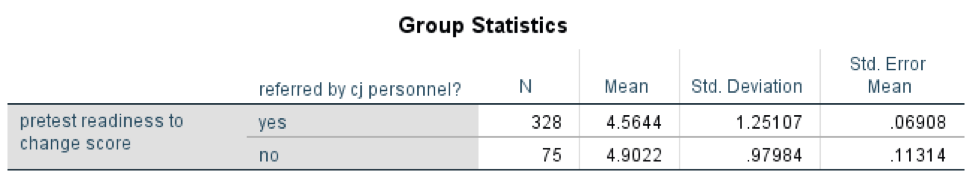
This table shows the mean value on readiness to change scores for the 328 men court-ordered to treatment was 4.56 and the mean for the 75 who entered the program voluntarily was 4.90 (with rounding). Clearly the difference between these two groups is not exactly zero: there exists a 0.34-point difference between the two group means (4.90 – 4.56 = 0.34). But is this 0.34-point difference observed in the sample sufficiently far from zero for investigators to reject the null hypothesis of there being no difference and to conclude that a population difference exists? This is another way of asking if the difference from zero is statistically significant.
The investigators in this case could use a t-test analysis approach for comparing the two group means (more about this later). The observed 0.34 difference in the two group means was significant at the p=0.029 level (probability=.03 with rounding) in this analysis. How does this translate into a conclusion about the results?
- The investigators adopted the tradition of using α=.05 criterion as a decision rule—accepting a 5% chance of drawing the wrong conclusion, being 95% confident of their conclusion.
- The computed statistical significance for the difference between the groups was 0.03 (rounding the p=0.029 level).
- The computed significance level (α=.03) is less than the accepted α=.05 criterion value, so the decision is to reject the null hypothesis of no difference (concluding that a difference exists).
- Additionally, the confidence interval for the sample t-statistic did not include the value 0, since both the lower and upper range values were negative numbers/less than zero: CI95%= (-.641, -.034). Thus, the investigators are 95% certain that the real population difference does not include zero as a possibility and rejected the null hypothesis of no difference: the conclusion is that a statistically significant association between program entry status (voluntary versus court order) and readiness to change scores exists in the population of men entering batterer treatment programs.
- Looking at the observed sample means shows that individuals entering the programs voluntarily had higher readiness to change scores than did individuals court-ordered to enter the programs (M=4.90 and 4.56 respectively). This could be reported as the voluntary entry group has significantly higher mean readiness to change scores than the group entering treatment through court order.
One-tailed and Two-tailed Hypotheses. Up until this point, we have worked with testing hypotheses about a “difference.” The difference could be in either direction, either group being more or less than the other. For example, an alternative hypothesis (Ha) could be:
Ha: A significant difference exists in the readiness to change scores between men voluntarily entering batterer treatment and men court-ordered to treatment.
In this case, the null hypothesis (H0) being statistically tested would be:
H0: No significant difference exists in the readiness to change scores between men voluntarily entering batterer treatment and men court-ordered to treatment (the difference is zero.)
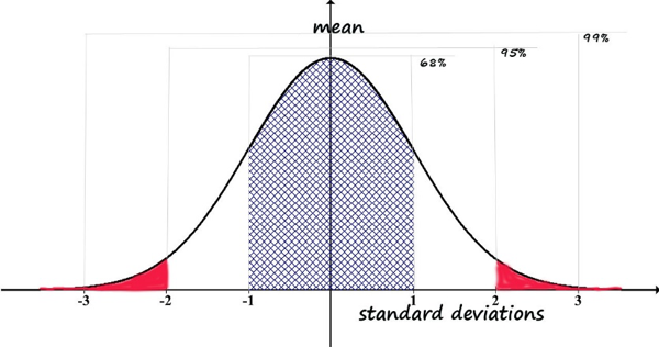
This null hypothesis could be rejected in either of two scenarios: either the voluntary entry group has higher readiness to change scores OR the voluntary entry group has lower readiness to change scores compared to the court-ordered group. In statistical terms, this means that we would be working with the probability of the result being either in the 2.5% tail above the mean or in the 2.5% tail below the mean (if we apply the α=.05 decision rule). This is what is meant by a two-tailed test—the null hypothesis would be rejected by a result landing in either of the two tails (values falling in either of the red areas of the curve below); values landing anywhere else would result in failure to reject the null hypothesis.
However, there exists another possible alternative hypothesis (Ha), depending on what the investigators think about the research question:
Ha: the voluntary entry group’s readiness scores will be significantly greater than the court-ordered group’s scores.
This changes the null hypothesis (H0) to the following:
H0: the voluntary entry group’s readiness scores will not be significantly greater than the court-ordered group’s scores.
Now there is only one tail that can lead to rejecting the null hypothesis: the resulting statistic would have to be in the 2.5% at the top tail of the distribution to reject. If it is in the 95% middle or in the bottom 2.5%, the investigator would fail to reject this null hypothesis. Since there is only one way to reject this time, not two, this is called a one-tail test (rejecting the null hypothesis for values falling in the red area of the curve, failing to reject the null hypothesis for values falling anywhere else).
In summary, if the hypothesis is directional, the decision rule needs to be based on one-tailed test criteria; if the hypothesis is bi-directional (difference could be either way), the decision rule should be based on two-tailed test criteria.
Type I and Type II Error
While the investigators in our Safe At Home example would be happy to share their results and conclusions with the world, it is important to understand the possibility that their conclusions could have been drawn in error. Remember: being 95% confident means accepting a 5% probability of being wrong (α=.05 criterion). In any situation, 4 possible combinations of decisions and realities exist: two represent accurate decisions and two represent mistaken decisions. The mistake possibilities include a Type I error and a Type II error (see Figure 4-2 adapted from Begun, Berger, & Otto-Salaj, 2018, p. 13) depending on whether the investigator rejects or fails to reject the null hypothesis.
Figure 4-2. Type I and Type II errors for the null hypothesis (H0=no difference)
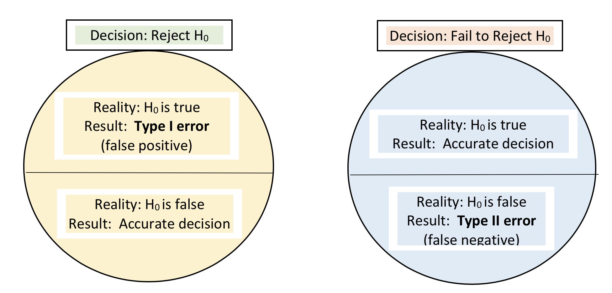
Type I Error. The risk of making a Type I error concerns the risk of rejecting the null hypothesis of no difference when in reality there exists no significant difference in the population. For example, our Safe At Home investigator rejected the null hypothesis of no difference in readiness to change scores between the two groups. A Type I error would occur if, in fact, there is no difference in readiness to change within the population of men entering batterer treatment programs.
Sometimes, investigators decide to apply a looser criterion: α=.10 means a 10% chance of being wrong, or 90% confidence. This would increase the probability of making a Type I error since it is “easier” to reject at this level. There are few instances in social work, social science, and behavioral research where 99% certainty is preferable to 95% certainty (α=.01 rather than α=.05). The reason being that we also want to reduce the probability of a Type II error.
Type II Error. The risk of making a Type II error concerns the risk of failing to reject the null hypothesis when, in reality, a significant difference in the population does exist. For example, if an investigator uses the α=.05 decision criterion and computes a significance value p=.06 from the sample data, the null hypothesis would not be rejected. In reality, however, a difference may truly exist in the population. This is problematic with intervention research conducted with too few study participants; with small samples it is harder to reject the null hypothesis. A very promising intervention may get “scrapped” as a result of a Type II error. Thus, study design is an important strategy for reducing the probability of making a Type II error.
Trochim (2005, p. 204) explains Type I and Type II error this way:
Type I Error: Finding a Relationship When There Is Not One (or Seeing Things That Aren’t There)
Type II Error: Finding No Relationship When There Is One (or Missing the Needle in the Haystack).
Take a moment to complete the following activity.
Chapter Summary
This chapter laid the groundwork for understanding inferential statistical approaches presented in Chapter 5. In this chapter you learned basic principles of probability and how these probability principles play a role in the logic and assumptions underlying inferential statistics. As a result, you should now have a basic understanding of the decision rules that are commonly applied in social work, social science, and behavioral statistics—the role of p and α, for example. You learned about the logic behind the null hypothesis (H0) and how it relates to a research question or “alternative” hypothesis (Ha),as well as what it means to reject or fail to reject the null hypothesis. You also learned about the distinction and meaning of Type I and Type II errors. Now you are prepared with a base for understanding specific statistical analyses.
