Module 4 Chapter 5: Introduction to 5 Statistical Analysis Approaches
Prior modules and chapters laid the groundwork for understanding the application of inferential statistics approaches commonly used to evaluate research hypotheses based on quantitative data. Inferential statistics may answer either univariate or bivariate hypotheses.
In this chapter, you will learn about:
- Specific statistical approaches for testing hypotheses (parametric tests of significance)
-
- one-samplet-test
- independent samples t-test
- one-way analysis of variance (Anova) test
- chi-square test of independence
- correlation test
-
- Approaches to consider when data are not normally distributed (non-parametric options)
What These Tests Have in Common
The five statistical analysis approaches presented here have several things in common. First, they each are based on a set of assumptions and/or have specific requirements related to the type of data analyzed. Second, with the exception of the chi-square test of independence, they rely on assumptions related to normal distribution in the population on at least one variable. Third, they all assume that the sample was randomly (properly) drawn from the population, and therefore are representative of the population. These last two factors characterize these are parametric tests (non-parametric tests are briefly discussed at the end of this chapter). For each of the statistical approaches, the task involves computing a test statistic based on the sample data, then comparing that computed statistic to a criterion value based on the appropriate distribution (t-distribution, F-distribution, χ2 distribution, or correlations). This comparison leads the investigator to either reject or fail to reject the null hypothesis.
One Sample t-Test
One of the simplest statistical tests to begin with allows investigators to draw conclusions based on a single group’s data about whether the population mean for the group is different from some known or expected standard mean value. For example, the standard IQ test has a mean value of 100—the test is designed so that the population is approximately normally distributed for IQ around this mean. Imagine that an investigator has concerns that a specific group in the population—perhaps children living in rental households—has a mean IQ significantly different from that standard mean of 100. In theory, this could happen from children being exposed to environmental toxins, such as lead in drinking/cooking water, and ingesting particles contaminated by lead-based paint or playground soil contaminated from heavy traffic where lead was once in the gasoline of cars driving in the area.

Test Purpose: Assess the probability that the population subgroup’s mean IQ differs from the standard population mean of 100.
Test H0: The group’s mean IQ is not significantly different from 100.
Type of Data: IQ scores are interval data.
Test Assumptions and Other Test Requirements: The univariate one-sample t-test is based on the following assumptions and requirements.
- Type of Variable: The scale of measurement is either ordinal or continuous (interval).
- Normal Distribution: The dependent variable is normally distributed in the population, or a sufficiently large sample size was drawn to allow approximation of the normal distribution.
- Independent Observations: Individuals in the sample are independent of each other—random selection indicates that the chances of one being sampled are independent of the chances for any other being sampled.
The test statistic: The t-test analysis is based on the t-distribution. The t-statistic is computed by first subtracting from the sample mean (X̅) the comparison value called “delta” (delta is indicated by the symbol Δ, which in our example has Δ = 100), then dividing this resulting value by the value computed as the sample’s standard deviation (s) multiplied by a fraction with 1 divided by the square root of the sample size. The formula looks like this:
t(df)= (X̅ – Δ)/[(s) * 1/√n)]
It should remind you somewhat of the formula we saw back in Chapter 3 for the 95% confidence interval using the t-value—we are using the same components of sample mean (X̅), t-value, standard deviation (s), and the square root of the sample size (√n):
CI95% = X̅ + [(tfor 95% confidence) * (s/√n)] (computes highest value)
CI95% = X̅ – [(tfor 95% confidence) * (s/√n)] (computes lowest value
Completing the example:In our hypothetical example, imagine the following: our sample mean (X̅)for IQ was 92, the standard deviation (s) was 21.00, and the sample size was 49 children. This means that our degrees of freedom (df) is 49 -1, or 48 (because df=n-1). We can consult the t-distribution table (from Chapter 3) to determine our decision value for t-values based on 48 degrees of freedom and α=.05 (95% confidence). Since our table does not show a value for 48 degrees of freedom, we estimate the criterion value as 2.01 for purposes of our example.
Plugging these values into the formula, we obtain our t-value:
t(48)= (92 -100)/ (21.00/√49)
t(48)= (-8)/ (21.00/7)
t(48)= (-8)/3
t(48)= (-2.67)
Now, we take that t(48)= -2.67 value and compare it to the criterion value from the t-distribution table (2.01). Since 2.67 (the “absolute value” of -2.67) is more extreme than our criterion value of 2.01, we reject the null hypothesis of no difference. In other words, we conclude that a significant difference exists in the mean IQ score for this subpopulation compared to the expected standard mean of 100.
On the other hand, our statistical computations using the computer might have generated a p-value for this test. Instead of using the t-distribution table at 95% confidence to determine a criterion value for comparing the t-statistic we calculated, the p-value computation will lead to the same conclusion. In this example, imagine that the computer informed us that the probability of a chance difference (p-value) was .024: p=.024 in the output. Using the α=.05 decision criterion (95% confidence), we see that .024 is less than .05. Thus, we reject the null hypothesis of no difference, just as we did using the t-statistic compared to the criterion value.
Note: we used a two-tailed test in this example. If the investigator hypothesized that the subgroup has a lower IQ than the mean, one-tailed test criteria would need to be applied.
Interactive Excel Workbook Activities
Complete the following Workbook Activity:
Comparing Means for Two Groups: Independent Samples t-Test
The next level of complexity involves comparing the mean for two independent groups, rather than what we just saw in comparing a single group to a standard or expected value. This moves us into a bivariate statistical analysis approach: one independent and one dependent variable. The independent variable is the “grouping” variable, defining the two groups to be compared. The dependent variable is the “test” variable, the one on which the two groups are being compared.
For example, we have been working throughout the module with the question of whether there is a meaningful difference in readiness to change scores for clients entering batterer treatment voluntarily versus through court order. In this case, we have one interval variable (readiness to change score) and one categorical variable with 2 possible categories—a dichotomous variable (entry status).
Test Purpose: Assess the probability that the readiness to change score in the population of clients entering batterer treatment voluntarily differs from the change scores for the population of clients entering batterer treatment through a court order.
Test H0: The mean readiness to change scores for the two groups are not significantly different (the difference equals zero).
Type of Data: Independent “grouping” variable (entry status) is both categorical and dichotomous; dependent variable (readiness to change scores) is interval data.
Test Assumptions and Other Test Requirements: The independent samples t-test is based on the following assumptions and requirements.
- Type of Variable: The scale of measurement for the dependent variable is continuous (interval).
- Normal Distribution: The dependent variable is normally distributed in the population, or a sufficiently large sample size was drawn to allow approximation of the normal distribution. Note: the “rule of thumb” is that neither group should be smaller than 6, and ideally has more.
- Independent Observations: Individuals within each sample and between the two groups are independent of each other—random selection indicates that the chances of any one “unit” being sampled are independent of the chances for any other being sampled.
- Homogeneity of Variance: Variance is the same for the two groups, as indicated by equal standard deviations in the two samples.
The test statistic: The independent samples t-test analysis is based on the t-distribution. The t-statistic is computed by first computing the difference between the two groups’ means: subtracting one mean (X̅courtorder)from the other (X̅voluntary). This computed difference is then divided by a sample standard deviation value divided by the square root of the sample size, just as we did in the one mean test. However, this is more complicated when we have two groups: we need a pooled estimate of the variance (a pooled standard deviation) since neither standard deviation alone will suffice. Furthermore, we need a pooled sample size since both groups 1 and 2 contributed to the variance estimate. Our earlier formula looked like this:
t(df)= (X̅ – Δ)/[(s) * 1/√n)]
Our new formula looks like this:
t(df)= (X̅1 – X̅2)/[(spooled) * 1/√n1+ 1/√n2).
Before we can start plugging in values, we need to know how to find the pooled variance estimate—the pooled standard deviation. The pooled standard deviation is computed as a sort of weighted estimate, with each group contributing the proportion of variance that is appropriate for its sample size—the smaller group contributing less to the estimate than the larger group. Thus, s1 is the standard deviation for group 1, and s2 is the standard deviation for group 2. Making a series of mathematical adjustments for the equivalent aspects of multiplying and dividing fractions, we end up with a formula for the pooled standard deviation (sp) that works like this:
- take the square root of the entire computed value where
- the first group’s degrees of freedom (sample size minus one, or n1-1) is multiplied by its standard deviation (s12) and
- this is added to the second group’s degrees of freedom (n2-1)multiplied by its standard deviation (s22)
- and that addition becomes the numerator of a fraction where the two sample sizes are added, and the 2 extra degrees of freedom are subtracted (n1+ n2-2)
In terms of a mathematical formula, it looks like this:
sp= √[(n1-1)*s12+ (n2-1)*s22/ (n1 + n2 – 2)]
Then, we take this pooled standard deviation and plug it into the t-test formula above. The degrees of freedom for this t-statistic will be the (n1+ n2– 2) that was in the denominator of our pooled variance.
Completing the example: The first step is to compute the pooled standard deviation value, then plug it into the formula for computing the t-statistic. In lieu of calculating this by hand, we can let Excel or another statistical program perform the calculation. The resulting t-statistic for comparing the mean readiness to change scores for our two groups, where the degrees of freedom were 401 (df=401):
t(401)= 2.189
The criterion value for 95% confidence was 1.960 in the t-distribution table. Therefore, the decision would be to reject the null hypothesis of equal means. The mean for the voluntary group was greater than the mean for the court order group: X̅=4.90 and X̅=4.56 respectively, a difference in the means of .34 (X̅1– X̅2= 4.90 – 4.56 = .34).
Two other ways of drawing the same conclusion (reject the null hypothesis) are offered by the computer output. The analysis indicated a 95% confidence interval of the difference in the two group means (.34) does not include zero as a possible value since the range includes only positive values: CI95% = (.64, .03). In addition, the two-tailed significance level computed for the test statistic (t-value) was p=.029. Using the criterion of α=.05, seeing that .029 is less than .05, the same conclusion is drawn: reject the null hypothesis of no difference between the groups. All three of these approaches came to the same conclusion because they are simply different ways of looking at the very same thing.
Interactive Excel Workbook Activities
Complete the following Workbook Activity:
Comparing Means: One-Way Analysis of Variance (Anova) Test
The one-way analysis of variance (Anova) test is another bivariate statistical analysis approach. Like the independent samples t-test, it is used to compare the means on an interval (continuous) variable for independent groups. Unlike the independent samples t-test, it is not restricted to comparing only 2 groups. For example, the one-way analysis of variance would allow an investigator to compare the means between multiple racial/ethnic groups, or between 3 treatment conditions (e.g., low, medium, high dose intervention groups, or treatment innovation, treatment as usual, no treatment control groups). In this case, we still have a bivariate statistical analysis approach: one independent and one dependent variable. The independent variable is still the “grouping” variable, defining two or more groups to be compared. The dependent variable is the “test” variable, the one on which the groups are being compared.
Two points are worthy of noting here. First, because they are mathematically related, the one-way Anova test, when conducted on a dichotomous (two-group) categorical variable yields a result identical to the independent samples t-test. The F-statistic is the square of the t-statistic in this 2-group case, and the F-distribution (as well as the criterion value) are squared, as well. Thus, the conclusion drawn and the p-value are identical.
Second, in a one-way Anova involving three or more groups, the result indicates whether a difference in mean values exists—it does not indicate where the difference lies. For example, it could be that one group differs from all the others, that all of the groups differ from each other, or some combination of differences and no differences. A significant result leads to further “post hoc” analyses to determine which pairs differ significantly.
Extending our example with readiness to change scores for men entering batterer treatment, consider the possibility that investigators wanted to explore the relationship between readiness to change scores and substance use at the time of the referring incident of intimate partner violence. The “grouping” independent variable was coded for who used substances at that time: (0) substances were not involved, (1) the client only, (2) the partner only, and (3) both client and partner. Thus, the analysis involves 4 groups being compared on the dependent variable (readiness to change battering behavior).
Data were available on both the dependent and independent variables for 391 clients. Here is what the mean and standard deviations looked like, as well as the 95% confidence interval for each group mean (see Table 5-1).
Table 5-1. Results of descriptive analyses for group means.
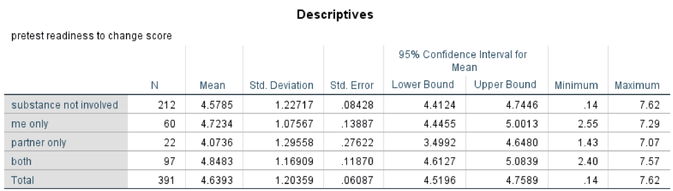
You can see the number of individuals in each group under the column labeled “N” and the mean readiness to change score for each group in the next column (labeled “Mean”). The group with the highest mean score was the group where both partners were using alcohol or other substances at the time of the incident, followed by the group where the client was the only one using at the time. The lowest readiness to change scores were among men whose partner was the only one using alcohol of other substances at the time of the incident, lower than the group where no substances were used by either partner. The 95% confidence intervals for these mean values all excluded zero as a possibility, since lower and upper bounds of the confidence interval (range) were positive values.
Test Purpose: Assess the probability that the readiness to change scores differ for the population of clients entering batterer treatment following an incident of intimate partner violence where no substances, client only substance use, partner only substance use, or both using substances was involved.
Test H0: The mean readiness to change scores for the four groups are equal (the differences equal zero). As previously noted, this multi-group test will not tell us which groups differ from the others, only whether there exists a difference to further analyze.
Type of Data: Independent “grouping” variable (substance use status) is categorical; dependent variable (readiness to change scores) is interval data.
Test Assumptions and Other Test Requirements: The one-way analysis of variance (Anova) test is based on the following assumptions and requirements.
- Type of Variable: The scale of measurement for the dependent variable is continuous (interval).
- Normal Distribution: The dependent variable is normally distributed in the population, or a sufficiently large sample size was drawn to allow approximation of the normal distribution. Note: the “rule of thumb” is that no group should be smaller than 7, and ideally each group has more.
- Independent Observations: Individuals within each sample and between the different groups are independent of each other—random selection indicates that the chances of any one “unit” being sampled are independent of the chances for any other being sampled.
- Homogeneity of Variance: Variance is the same for each group, as indicated by equal standard deviations in the groups’ samples.
The test statistic: The Anova test analysis is based on the F-distribution. The F-statistic is computed as a complex difference value divided by a complex value computed with standard deviations and group sample sizes. This is the same logic used in our t-statistic computation, just more complexly computed because there are more groups involved. The F-statistic is then compared to the criterion values for the F-distribution, the same way we did this comparison using the t-distribution to find the criterion t-statistic values. It is beyond the scope of this course to compute the F-statistic manually; it is sufficient to understand what it means.
One important facet of the F-statistic evaluation is understanding the degrees of freedom involved. In fact, with the F-statistic there are two different types of degrees of freedom involved: between groups and within group degrees of freedom. Between groups degrees of freedom is related to the number of groups, regardless of group size. In our example involving 4 groups, the between groups degrees of freedom is 4-1, or df=3. Within groups degrees of freedom is related to the number of individuals in the entire sample, but instead of being n-1, it is n minus the number computed for between groups degrees of freedom. In our example with data provided by 390 men from 4 groups, the within groups degrees of freedom is 390 – (4-1) = 387. This is written as df=(3,387)—this is not read as three thousand three hundred eighty seven degrees of freedom, it is read as 3 and 387 where the first number is always the between groups degrees of freedom and the second number is always the within groups degrees of freedom.
Completing the example: The next task is to apply our computed degrees of freedom to an F-distribution table to determine the criterion value for df=(3, 387) at 95% confidence (α=.05): this turns out to be a criterion value of 2.60. Then, we allow the computer to generate the comparison F-statistic for our data, as presented in this table (see Table 5-2).
Table 5-2. Results of one-way analysis of variance, 4 group mean readiness to change scores.
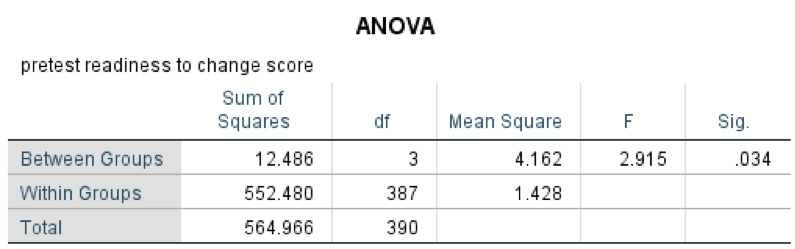
The values in the Sum of Squares and Mean Square cells relate to what would be plugged into the formula that we are not delving into in this course. The F-statistic computation answer would be written as F(3, 387)=2.92, p=.034 for this analysis. Therefore, the decision would be to reject the null hypothesis of equal means since the F-statistic value of 2.92 is greater than the criterion value of 2.60 from the F-distribution table.
Another way of drawing the same conclusion (reject the null hypothesis) is offered by the computer output. The analysis indicated a significance level computed for the test statistic (F-statistic) was p=.034. Using the criterion of α=.05, seeing that .034 is less than .05, the same conclusion is drawn: reject the null hypothesis of equal means. Both of these approaches came to the same conclusion because they are simply different ways of looking at the very same thing. Post-hoc comparisons would be required to determine which of the differences in means listed in Table 5-1 are significantly different; remember that the test only told us that a statistically significant difference exists .
Interactive Excel Workbook Activities
Complete the following Workbook Activity:
Chi-square Test of Independence
The chi-square test (often written as the χ2test, pronounced “chi-square”) is a bivariate statistical analysis approach. It is used to evaluate whether a significant relationship exists between two categorical (nominal) variables. Data are conceptualized in the format of a contingency table (see Table 5-3), where the categories for one of the two variables are represented as rows and categories for the other variable are represented as columns. The chi-square test is concerned with analyzing the relative proportions with which cases from the sample are sorted into the different cells of the contingency table.
For example, we can look at the Safe At Home data concerning whether there exists a significant relationship between treatment entry status (voluntary or court order) and treatment completion (completed or dropped out). The data would be entered into a 2 x 2 contingency table, where Oi is the observed number of cases in each cell, with i being 1, 2, 3, or 4 depending on which cell is being identified (see Table 5-3).
Table 5-3. Contingency table for chi-square analysis of treatment entry status and treatment completion.
| Program Completion | ||||
|---|---|---|---|---|
| yes (completed) | no (dropped) | row total | ||
| Entry Status | court-ordered | O1 | O2 | |
| voluntary | O3 | O4 | ||
| column total | ||||
Test Purpose: Assess the independence of treatment entry status and treatment completion variables.
Test H0: No association between the variables exists (i.e., the variables are independent of each other if differences in the cell proportions equal zero).
Type of Data: Two variables are categorical, with two or more possible categories each.
Test Assumptions and Other Test Requirements: The chi-square test is based on the following assumptions and requirements.
- Type of Variable: The scale of measurement for both variables is categorical (nominal).
- Distribution: Normal distribution is not assumed with categorical variables. The χ2-distribution is used to evaluate the test statistic.
- Independent Observations :Individuals within each sample and between the different groups are independent of each other—random selection indicates that the chances of any one “unit” being sampled are independent of the chances for any other being sampled.
- Estimating Expected Cell Counts: In order to compute the χ2-test statistic, the number of cases expected in each cell of the contingency table if the two variables are independent of each other must be calculated; this requires sufficient sample size and a minimum of 5 expected cases per cell.
The test statistic: The chi-square test analysis is based on the χ2-distribution. The χ2-test statistic is computed in terms of the observed counts in each cell compared to what would be the expected counts if no relationship exists between the two variables. In essence, the formula for computing the χ2-test statistic is relatively simple: for each cell, compute the difference between what was observed and what was expected, square the difference, and divide the result by the expected value for that cell; then, add up the results for the individual cells into a single value. In mathematical terms, the formula looks like this:
χ2= ∑(Oi– Ei)2 / Ei
- χ2 is the relevant test-statistic
- the ∑ symbol means add the values up (compute the sum)
- Oi is the observed number in the ith cell (i designates each cell in the contingency table; 1 through 4 in a 2×2 table; 1 through 6 in a 2 x 3 table; 1 through 9 in a 3×3 table; and so forth)
- Ei is the expected number in the ith cell (i designates each cell in the contingency table; 1 through 4 in a 2×2 table; 1 through 6 in a 2 x 3 table; 1 through 9 in a 3×3 table; and so forth)
The only thing we still need to know is how to calculate the expected (Ei) value for each of the contingency table cells. Again, this is a simple calculation based on the row, column, and sample size total values related to each cell.
Ei= (row total * column total)/sample size
Completing the Example: In the Safe At Home study example investigators wanted to know if there exists an association between program entry status and program completion. (The null hypothesis being tested is that no association exists; that the two variables are independent of each other). Table 5-4 presents the completed 2 x 2 contingency table with the observed (Oi) values are presented, as are the calculated expected (Ei)values for each cell.
Table 5-4. Data distribution for chi-square analysis of treatment entry status and treatment completion.
| Program Completion | ||||
|---|---|---|---|---|
| yes (completed) | no (dropped) | row total | ||
| Entry Status | court-ordered | O1 = 174 E1 = 173.7 |
O2 = 234 E2 = 234.3 |
408 |
| voluntary | O3 = 38 E3 = 38.3 |
O4 = 52 E1 = 51.7 |
90 | |
| column total | 212 | 286 | 498 | |
- O1 is court-ordered clients completing treatment: E1=(212 * 408)/498=173.7
- O2 is court-order clients dropping out of treatment: E2=(286 * 408)/498=234.3
- O3 is voluntary clients completing treatment: E3=(212 * 90)/498=38.3
- O4 is voluntary clients dropping out of treatment: E4=(286 * 90)/498=51.7
We now have all the information necessary for computing the χ2-test statistic.
χ2= ∑(Oi– Ei)2/Ei
χ2=[(174-173.7)2/173.7]+[(234-234.3)2/234.3]+[(38-38.3)2/38.3]+[52-51.7)2/51.7]
χ2=[.32/173.7]+[-.32/234.3]+[-.32/38.3]+[.32/51.7]
χ2=[.09/173.7]+[.09/234.3]+[.09/38.3]+[.09/51.7]
χ2=.00052 + .00038 + .0023 + .0017
χ2=.0049
What remains is to evaluate the χ2-test statistic which we computed as .005 (with rounding up from .0049). This value can be compared to the criterion value for χ2-distribution based on the degrees of freedom at α=.05. In order to do so, we need to know the degrees of freedom for this analysis. In general, degrees of freedom for a chi-square test are computed as the number of rows minus 1 and the number of columns minus 1. In a mathematical formula, this would be:
df=(#rows-1, #columns-1).
Thus, for our 2 x 2 contingency table, the degrees of freedom would be 2-1 = 1 for each, rows and columns: we would write this as df=(1,1). The criterion value is then looked up in a chi-square distribution table. For df=(1,1) at 95% confidence (α=.05), the criterion value is 3.841. In our example, the computed .005 is less than the criterion value, therefore we fail to reject the null hypothesis. In other words, there could very well be no association between the two variables—they could be operating independently of each other.
Another way of drawing the same conclusion is to have computed the probability value (p-value) for our analysis. In this case, the statistical program computed a p-value of .941 for our χ2-test statistic. Because .941 is greater than our decision rule of α=.05, we fail to reject the null hypothesis.
Interactive Excel Workbook Activities
Complete the following Workbook Activity:
Correlation Test
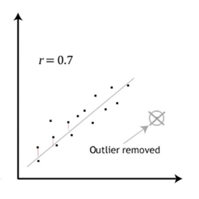
Correlation is used to analyze the strength and direction of a linear relationship between two interval (continuous) variables. Similar to the chi-square test, it assesses the probability of a linear association between the two variables, but in this case the variables are not categorical, they are interval numeric variables. The correlation analysis involves determining the single line that best fits the observed sample data points. In other words, the line which has the shortest possible total of distances each point lies from that line. Figure 5-1 shows just such a line drawn through hypothetical data and the first few distances from data points to that line are shown in red. The goal is to find the line where the total of those distances is the least possible.
Figure 5-1. Best line through data points with correlation coefficient 0.7, with one outlier removed. (Note: image adapted from https://statistics.laerd.com/spss-tutorials/pearsons-product-moment-correlation-using-spss-statistics.php)
The correlation coefficient is designated in statistics as r. The value for rcommunicates two important dimensions about correlation: strength of the association or relationship between the two variables and direction of the association.
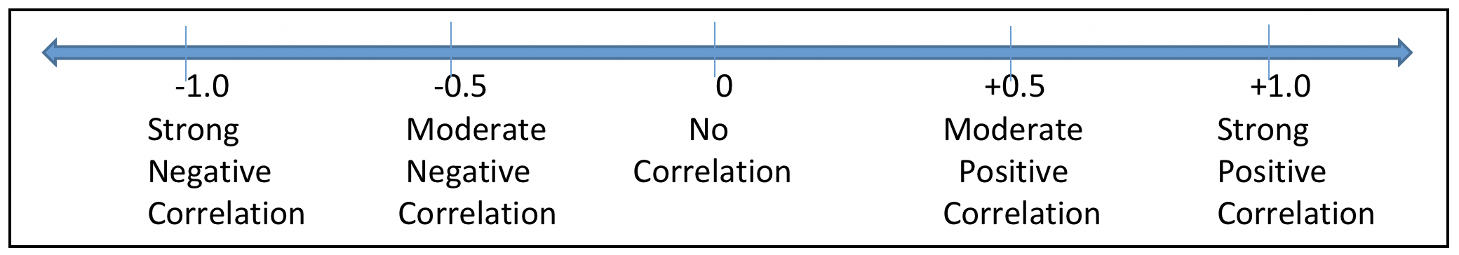
Strength of Relationship. The possible range of the correlation coefficient is from -1 to +1. If two variables have no linear relationship to each other, the correlation coefficient is 0. A perfect correlation between two variables would be either -1 or +1—in other words, the absolute value ofris 1. Neither of these extremes usually happens, so the strength of the association is determined by how far from zero the correlation coefficient (r) actually lies. This diagram might help you visualize what this means:
The histograms we saw in Chapter 2 depicted univariate data—the frequency with which specific values on a single variable were represented in the sample data. Bivariate analyses are depicted using a scatterplot where each data point (dot) on the scatterplot indicates an individual participant’s value on each of two variables, the x-variable and they-variable (height and weight, for example). Figures 5-2 and 5-3 graphically depict hypothetical examples of data points with zero or no correlation (no evident line) and a perfect +1 correlation.
Figure 5-2. Hypothetical scatterplot with no correlation.
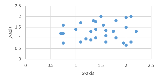
Figure 5-3. Hypothetical scatterplot with perfect +1 correlation (45o angle line).
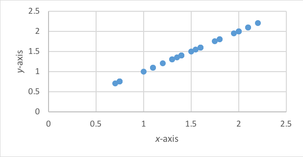
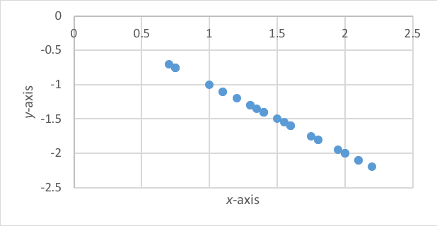
Direction of Association. There is a meaningful difference between a negative and a positive correlation coefficient. A perfect positive correlation of +1, as seen in Figure 5-2 indicates that as the values of one variable increase (x-axis), so do the values of the other variable (y-axis). On the other hand, a perfect negative correlation of -1 would indicate that as the values of one variable increase (x-axis), the values of the other variable decrease (y-axis). The perfect negative correlation is presented in Figure 5-4.
Figure 5-4. Hypothetical scatterplot with perfect -1 correlation (45o angle line).

Take a moment to complete the following activity.
Test Purpose: Assess the strength and direction of association between two variables.
Test H0: The two variables are unassociated in the population (i.e., their correlation is 0).
Type of Data: Both variables are interval for a Pearson correlation; if either/both is ordinal, a Spearman correlation is preferable.
Test Assumptions and Other Test Requirements: Correlation tests require the following conditions and the following considerations.
- Each case analyzed must have complete data for both variables; if more than one correlation is computed (multiple pairs of variables), cases can be deleted from the analysis wherever this is not true (pairwise deletion) or can be deleted from all analyses (listwise deletion).
- Data on each variable should be approximately normally distributed.
- Data should be assessed for “outliers” (extreme values) which can affect the correlation analysis. Outlier cases, typically having values more than 3.25 standard deviations from the mean (above or below), should be excluded from correlation analysis.
- Distribution of the data should be in a relatively tubular shape around a straight line drawn through the data points on a scatterplot; for example, a cone shape violates this assumption of homoscedascity. Homoscedascity refers to the degree of variance around the line being similar regardless of where along the x-axis the points are mapped. A cone shape would mean that low values on the xvariable have data points closer to the line than high values on the xvariable (a case of heteroscedascity).
- Distribution of data should be relatively linear. For example, a curved line reflects a non-linear relationship between the variables. Non-linearity violates an assumption necessary for correlation analysis.
- Statistically significant correlation coefficients are increasingly likely as sample sizes increase. Therefore, caution must be used in interpreting relatively low correlation coefficients (below about 0.3) which are flagged as statistically significant if the sample size is large.
- Correlation simply indicates an association between two variables, it does not in any way indicate or confirm a causal relationship between those variables. Always remember that correlation does not imply causality (you have read this before in other modules). Causal relationships require different kinds of study designs and statistical analyses to confirm.
The test statistic: As previously noted, correlation analysis is based on identifying from among an infinite array of possible lines, the one line that best defines the observed data—the line where the cumulative distance from data points to that line is minimized. The formula looks more complicated than it actually is. The correlations coefficient (r) is computed from a numerator divided by a denominator, just as our previous coefficients have been. The numerator is made up of the sample size N (the number of pairs for the two variables) multiplied by the sum of each pair of values (x times y for each case, summed) minus the result of multiplying the sum of the x values times the sum of the y values. The denominator is the square root of multiplying two things together: first, the sample size N times the sum of the x2 values minus the square of the sum of the x values, then doing the same for the y values—sample size N times the sum of the y2 values minus the square of the sum of the y values. In a mathematical formula, it looks like this, where the final step will be dividing the numerator by the denominator:
r numerator = N * ∑x*y – (∑x)*(∑y)
r denominator = square root of [N*∑x2 – (∑x)2] * [N*∑y2 – (∑y)2]
With large numbers of cases, hand calculating this correlation coefficient is cumbersome—computer software programs can do the computation very quickly.
Completing the example:Consider for example that the Safe At Home project investigators wanted to assess the association between readiness to change scores and the length of time between client entry into the treatment program and the intimate partner violence incident leading to treatment entry (measured in weeks). In our example, the computed correlation coefficient was r=-.060 for N=387 clients entering batterer treatment for whom completed data were available and following removal of three outliers with extremely long time lag between the incident and program entry.
The negative sign on the correlation coefficient suggests that greater number of weeks between incident and program entry might be associated with lower readiness to change scores. This could be explained in several different causal models, so it is not acceptable to infer that one caused the other:
- More time passing leads to less impetus to change.
- Low impetus to change leads to longer lag time before entering a program.
- Some other factor or factors influence both time to program entry and readiness to change scores.
The strength of the correlation coefficient needs to be assessed. The coefficient is not far from zero (.06 is not even 1/10th of the way to 1.0), suggesting that the association is weak. This is particularly notable since the sample size was so large (N=387): even a small correlation should be more easily detected with a large sample size. Allowing us to reject the null hypothesis is the computed two-tailed significance value where p=.241. Since .241 is greater than our decision rule of α=.05, we fail to reject the null hypothesis. In other words, we conclude that there may be no association between the two variables. In reality, this finding could be explained by some other factor or factors influencing the length of time before entering a program—events such as incarceration for the offenses could interfere with entering treatment, for example.
Interactive Excel Workbook Activities
Complete the following Workbook Activity:
Choosing the Right Statistical Test for the Job
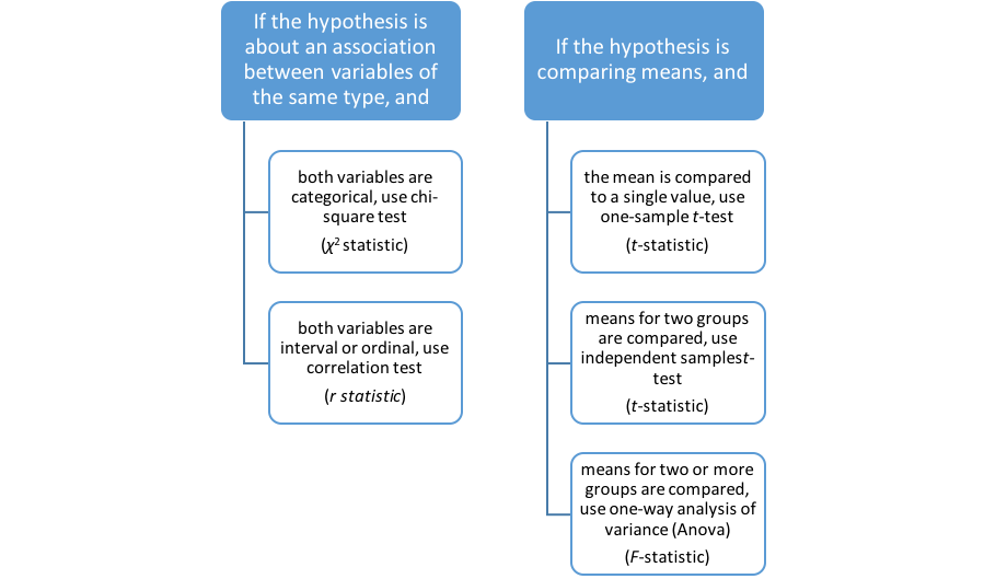
You have now been introduced to 5 powerful statistical tools for analyzing quantitative data. The guidelines for choosing the right tool for the job have to do with (1) the nature of the hypothesis being tested, and (2) the nature of the variables being analyzed. This flow chart might help (see Figure 5-5).
Figure 5-5. Decision flow chart for 5 statistical analytic approaches.
Take a moment to complete the following activity.
The Role of Non-Parametric Statistical Approaches
- Rank order all of the cases from lowest to highest on the dependent variable, regardless of which group they represent—all are in one single pool.
- Sum the ranks for one of the two groups (it does not matter which is selected)—this becomes R1 in the formula below.
- Compute the result of [number of cases in group1 * (number of cases in group1+1)] divided by 2.
- The test statistic is the result of subtracting this last computation from the R1 value.
