Module 3 Chapter 4: Overview of Quantitative Study Variables
The first thing we need to understand is the nature of variables and how variables are used in a study’s design to answer the study questions. In this chapter you will learn:
- different types of variables in quantitative studies,
- issues surrounding the unit of analysis question.
Understanding Quantitative Variables
The root of the word variable is related to the word “vary,” which should help us understand what variables might be. Variables are elements, entities, or factors that can change (vary); for example, the outdoor temperature, the cost of gasoline per gallon, a person’s weight, and the mood of persons in your extended family are all variables. In other words, they can have different values under different conditions or for different people.
We use variables to describe features or factors of interest. Examples might include the number of members in different households, the distance to healthful food sources in different neighborhoods, the ratio of social work faculty to students in a BSW or MSW program, the proportion of persons from different racial/ethnic groups incarcerated, the cost of transportation to receive services from a social work program, or the rate of infant mortality in different counties. In social work intervention research, variables might include characteristics of the intervention (intensity, frequency, duration) and outcomes associated with the intervention.
Demographic Variables. Social workers are often interested in what we call demographic variables. Demographic variables are used to describe characteristics of a population, group, or sample of the population. Examples of frequently applied demographic variables are
- age,
- ethnicity,
- national origin,
- religious affiliation,
- gender,
- sexual orientation,
- marital/relationship status,
- employment status,
- political affiliation,
- geographical location,
- education level, and
- income.
At a more macro level, the demographics of a community or organization often includes its size; organizations are often measured in terms of their overall budget.
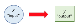
Independent and Dependent Variables. A way that investigators think about study variables has important implications for a study design. Investigators make decisions about having them serve as either independent variables or as dependent variables. This distinction is not something inherent to a variable, it is based on how the investigator chooses to define each variable. Independent variables are the ones you might think of as the manipulated “input” variables, while the dependent variables are the ones where the impact or “output” of that input variation would be observed.
Intentional manipulation of the “input” (independent) variable is not always involved. Consider the example of a study conducted in Sweden examining the relationship between having been the victim of child maltreatment and later absenteeism from high school: no one intentionally manipulated whether the children would be victims of child maltreatment (Hagborg, Berglund, & Fahlke, 2017). The investigators hypothesized that naturally occurring differences in the input variable (child maltreatment history) would be associated with systematic variation in a specific outcome variable (school absenteeism). In this case, the independent variable was a history of being the victim of child maltreatment, and the dependent variable was the school absenteeism outcome. In other words, the independent variable is hypothesized by the investigator to cause variation or change in the dependent variable. This is what it might look like in a diagram where “x” is the independent variable and “y” is the dependent variable (note: you saw this designation earlier, in Chapter 3, when we discussed cause and effect logic):
For another example, consider research indicating that being the victim of child maltreatment is associated with a higher risk of substance use during adolescence (Yoon, Kobulsky, Yoon, & Kim, 2017). The independent variable in this model would be having a history of child maltreatment. The dependent variable would be risk of substance use during adolescence. This example is even more elaborate because it specifies the pathway by which the independent variable (child maltreatment) might impose its effects on the dependent variable (adolescent substance use). The authors of the study demonstrated that post-traumatic stress (PTS) was a link between childhood abuse (physical and sexual) and substance use during adolescence.

Take a moment to complete the following activity.
Types of Quantitative Variables
There are other meaningful ways to think about variables of interest, as well. Let’s consider different features of variables used in quantitative research studies. Here we explore quantitative variables as being categorical, ordinal, or interval in nature. These features have implications for both measurement and data analysis.
Categorical Variables. Some variables can take on values that vary, but not in a meaningful numerical way. Instead, they might be defined in terms of the categories which are possible. Logically, these are called categorical variables. Statistical software and textbooks sometimes refer to variables with categories as nominal variables. Nominal can be thought of in terms of the Latin root “nom” which means “name,” and should not be confused with number. Nominal means the same thing as categorical in describing variables. In other words, categorical or nominal variables are identified by the names or labels of the represented categories. For example, the color of the last car you rode in would be a categorical variable: blue, black, silver, white, red, green, yellow, or other are categories of the variable we might call car color.
What is important with categorical variables is that these categories have no relevant numeric sequence or order. There is no numeric difference between the different car colors, or difference between “yes” or “no” as the categories in answering if you rode in a blue car. There is no implied order or hierarchy to the categories “Hispanic or Latino” and “Not Hispanic or Latino” in an ethnicity variable; nor is there any relevant order to categories of variables like gender, the state or geographical region where a person resides, or whether a person’s residence is owned or rented.
If a researcher decided to use numbers as symbols related to categories in such a variable, the numbers are arbitrary—each number is essentially just a different, shorter name for each category. For example, the variable gender could be coded in the following ways, and it would make no difference, as long as the code was consistently applied.
| Coding Option A | Variable Categories | Coding Option B |
|---|---|---|
| 1 | male | 2 |
| 2 | female | 1 |
| 3 | other than male or female alone | 4 |
| 4 | prefer not to answer | 3 |
Race and ethnicity.One of the most commonly explored categorical variables in social work and social science research is the demographic referring to a person’s racial and/or ethnic background. Many studies utilize the categories specified in past U.S. Census Bureau reports. Here is what the U.S. Census Bureau has to say about the two distinct demographic variables, race and ethnicity (https://www.census.gov/mso/www/training/pdf/race-ethnicity-onepager.pdf):
What is race? The Census Bureau defines race as a person’s self-identification with one or more social groups. An individual can report as White, Black or African American, Asian, American Indian and Alaska Native, Native Hawaiian and Other Pacific Islander, or some other race. Survey respondents may report multiple races.
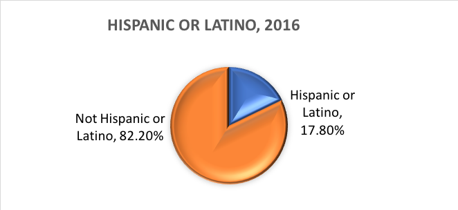
What is ethnicity? Ethnicity determines whether a person is of Hispanic origin or not. For this reason, ethnicity is broken out into two categories, Hispanic or Latino and Not Hispanic or Latino. Hispanics may report as any race.
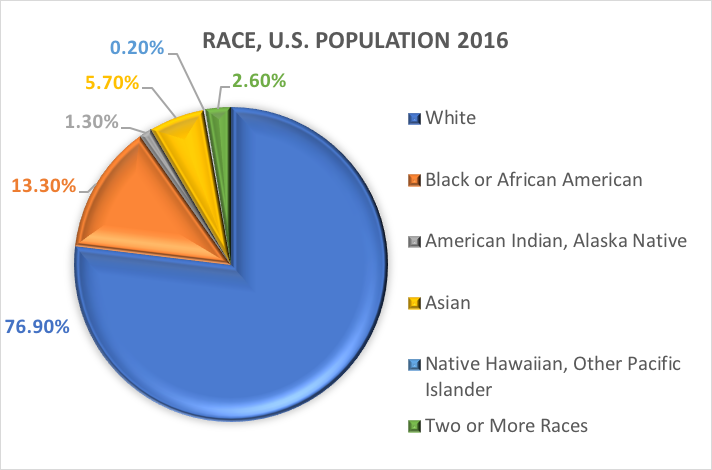
In other words, the Census Bureau defines two categories for the variable called ethnicity (Hispanic or Latino and Not Hispanic or Latino), and seven categories for the variable called race. While these variables and categories are often applied in social science and social work research, they are not without criticism.
Based on these categories, here is what is estimated to be true of the U.S. population in 2016:
Dichotomous variables.There exists a special category of categorical variable with implications for certain statistical analyses. Categorical variables comprised of exactly two options, no more and no fewer are called dichotomous variables. One example was the U.S. Census Bureau dichotomy of Hispanic/Latino and Non-Hispanic/Non-Latino ethnicity. For another example, investigators might wish to compare people who complete treatment with those who drop out before completing treatment. With the two categories, completed or not completed, this treatment completion variable is not only categorical, it is dichotomous. Variables where individuals respond “yes” or “no” are also dichotomous in nature.
The past tradition of treating gender as either male or female is another example of a dichotomous variable. However, very strong arguments exist for no longer treating gender in this dichotomous manner: a greater variety of gender identities are demonstrably relevant in social work for persons whose identity does not align with the dichotomous (also called binary) categories of man/woman or male/female. These include categories such as agender, androgynous, bigender, cisgender, gender expansive, gender fluid, gender questioning, queer, transgender, and others.
Ordinal Variables. Unlike these categorical variables, sometimes a variable’s categories do have a logical numerical sequence or order. Ordinal, by definition, refers to a position in a series. Variables with numerically relevant categories are called ordinal variables. For example, there is an implied order of categories from least-to-most with the variable called educational attainment. The U.S. Census data categories for this ordinal variable are:
- none
- 1st-4thgrade
- 5th-6thgrade
- 7th-8thgrade
- 9thgrade
- 10thgrade
- 11thgrade
- high school graduate
- some college, no degree
- associate’s degree, occupational
- associate’s degree academic
- bachelor’s degree
- master’s degree
- professional degree
- doctoral degree
In looking at the 2016 Census Bureau estimate data for this variable, we can see that females outnumbered males in the category of having attained a bachelor’s degree: of the 47,718,000 persons in this category, 22,485,000 were male and 25,234,000 were female. While this gendered pattern held for those receiving master’s degrees, the pattern was reversed for receiving doctoral degrees: more males than females obtained this highest level of education. It is also interesting to note that females outnumbered males at the low end of the spectrum: 441,000 females reported no education compared to 374,000 males.
Here is another example of using ordinal variables in social work research: when individuals seek treatment for a problem with alcohol misuse, social workers may wish to know if this is their first, second, third, or whatever numbered serious attempt to change their drinking behavior. Participants enrolled in a study comparing treatment approaches for alcohol use disorders reported that the intervention study was anywhere from their first to eleventh significant change attempt (Begun, Berger, Salm-Ward, 2011). This change attempt variable has implications for how social workers might interpret data evaluating an intervention that was not the first try for everyone involved.
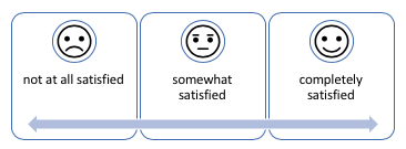
Rating scales. Consider a different but commonly used type of ordinal variable: rating scales. Social, behavioral, and social work investigators often ask study participants to apply a rating scale to describe their knowledge, attitudes, beliefs, opinions, skills, or behavior. Because the categories on such a scale are sequenced (most to least or least to most), we call these ordinal variables.
Examples include having participants rate:
- how much they agree or disagree with certain statements (not at all to extremely much);
- how often they engage in certain behaviors (never to always);
- how often they engage in certain behaviors (hourly, daily, weekly, monthly, annually, or less often);
- the quality of someone’s performance (poor to excellent);
- how satisfied they were with their treatment (very dissatisfied to very satisfied)
- their level of confidence (very low to very high).
Interval Variables. Still other variables take on values that vary in a meaningful numerical fashion. From our list of demographic variables, age is a common example. The numeric value assigned to an individual person indicates the number of years since a person was born (in the case of infants, the numeric value may indicate days, weeks, or months since birth). Here the possible values for the variable are ordered, like the ordinal variables, but a big difference is introduced: the nature of the intervals between possible values. With interval variables the “distance” between adjacent possible values are equal. Some statistical software packages and textbooks use the term scale variable: this is exactly the same thing as what we call an interval variable.
For example, in the graph below, the 1 ounce difference between this person consuming 1 ounce or 2 ounces of alcohol (Monday, Tuesday) is exactly the same as the 1 ounce difference between consuming 4 ounces or 5 ounces (Friday, Saturday). If we were to diagram the possible points on the scale, they would all be equidistant; the interval between any two points is measured in standard units (ounces, in this example).
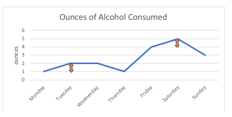
With ordinal variables, such as a rating scales, no one can say for certain that the “distance” between the response options of “never” and “sometimes” is the same as the “distance” between “sometimes” and “often,” even if we used numbers to sequence these response options. Thus, the rating scale remains ordinal, not interval.
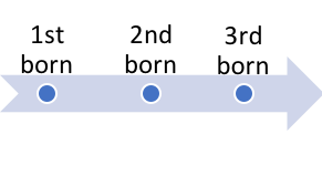
What might become a tad confusing is that certain statistical software programs, like SPSS, refer to an interval variable as a “scale” variable. Many variables used in social work research are both ordered and have equal distances between points. Consider for example, the variable of birth order. This variable is interval because:
- the possible values are ordered (e.g., the third-born child came after the first- and second-born and before the fourth-born), and
- the “distances” or intervals are measured in equivalent one-person units.
Continuous variables. There exists a special type of numeric interval variable that we call continuous variables. A variable like age might be treated as a continuous variable. Age is ordinal in nature, since higher numbers mean something in relation to smaller numbers. Age also meets our criteria for being an interval variable if we measure it in years (or months or weeks or days) because it is ordinal and there is the same “distance” between being 15 and 30 years old as there is between being 40 and 55 years old (15 calendar years). What makes this a continuous variable is that there are also possible, meaningful “fraction” points between any two intervals. For example, a person can be 20½ (20.5) or 20¼ (20.25) or 20¾ (20.75) years old; we are not limited to just the whole numbers for age. By contrast, when we looked at birth order, we cannot have a meaningful fraction of a person between two positions on the scale.
The Special Case of Income. One of the most abused variables in social science and social work research is the variable related to income. Consider an example about household income (regardless of how many people are in the household). This variable could be categorical (nominal), ordinal, or interval (scale) depending on how it is handled.
Categorical Example: Depending on the nature of the research questions, an investigator might simply choose to use the dichotomous categories of “sufficiently resourced” and “insufficiently resourced” for classifying households, based on some standard calculation method. These might be called “poor” and “not poor” if a poverty line threshold is used to categorize households. These distinct income variable categories are not meaningfully sequenced in a numerical fashion, so it is a categorical variable.
Ordinal Example: Categories for classifying households might be ordered from low to high. For example, these categories for annual income are common in market research:
- Less than $25,000.
- $25,000 to $34,999.
- $35,000 to $49,999.
- $50,000 to $74,999.
- $75,000 to $99,999.
- $100,000 to $149,999.
- $150,000 to $199,999.
- $200,000 or more.
Notice that the categories are not equally sized—the “distance” between pairs of categories are not always the same. They start out in about $10,000 increments, move to $25,000 increments, and end up in about $50,000 increments.
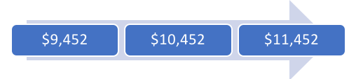
Interval Example. If an investigator asked study participants to report an actual dollar amount for household income, we would see an interval variable. The possible values are ordered and the interval between any possible adjacent units is $1 (as long as dollar fractions or cents are not used). Thus, an income of $10,452 is the same distance on a continuum from $9,452 and $11,452—$1,000 either way.
The Special Case of Age. Like income, “age” can mean different things in different studies. Age is usually an indicator of “time since birth.” We can calculate a person’s age by subtracting a date of birth variable from the date of measurement (today’s date minus date of birth). For adults, ages are typically measured in years where adjacent possible values are distanced in 1-year units: 18, 19, 20, 21, 22, and so forth. Thus, the age variable could be a continuous type of interval variable.
However, an investigator might wish to collapse age data into ordered categories or age groups. These still would be ordinal, but might no longer be interval if the increments between possible values are not equivalent units. For example, if we are more interested in age representing specific human development periods, the age intervals might not be equal in span between age criteria. Possibly they might be:
- Infancy (birth to 18 months)
- Toddlerhood (18 months to 2 ½ years)
- Preschool (2 ½ to 5 years)
- School age (6 to 11 years)
- Adolescence (12 to 17 years)
- Emerging Adulthood (18 to 25 years)
- Adulthood (26 to 45 years)
- Middle Adulthood (46 to 60 years)
- Young-Old Adulthood (60 to 74 years)
- Middle-Old Adulthood (75 to 84 years)
- Old-Old Adulthood (85 or more years)
Age might even be treated as a strictly categorical (non-ordinal) variable. For example, if the variable of interest is whether someone is of legal drinking age (21 years or older), or not. We have two categories—meets or does not meet legal drinking age criteria in the United States—and either one could be coded with a “1” and the other as either a “0” or “2” with no difference in meaning.
What is the “right” answer as to how to measure age (or income)? The answer is “it depends.” What it depends on is the nature of the research question: which conceptualization of age (or income) is most relevant for the study being designed.
Alphanumeric Variables. Finally, there are data which do not fit into any of these classifications. Sometimes the information we know is in the form of an address or telephone number, a first or last name, zipcode, or other phrases. These kinds of information are sometimes called alphanumeric variables. Consider the variable “address” for example: a person’s address might be made up of numeric characters (the house number) and letter characters (spelling out the street, city, and state names), such as 1600 Pennsylvania Ave. NW, Washington, DC, 20500.

Actually, we have several variables present in this address example:
- the street address: 1600 Pennsylvania Ave.
- the city (and “state”): Washington, DC
- the zipcode: 20500.
This type of information does not represent specific quantitative categories or values with systematic meaning in the data. These are also sometimes called “string” variables in certain software packages because they are made up of a string of symbols. To be useful for an investigator, such a variable would have to be converted or recoded into meaningful values.
A Note about Unit of Analysis
An important thing to keep in mind in thinking about variables is that data may be collected at many different levels of observation. The elements studied might be individual cells, organ systems, or persons. Or, the level of observation might be pairs of individuals, such as couples, brothers and sisters, or parent-child dyads. In this case, the investigator may collect information about the pair from each individual, but is looking at each pair’s data. Thus, we would say that the unit of analysis is the pair or dyad, not each individual person. The unit of analysis could be a larger group, too: for example, data could be collected from each of the students in entire classrooms where the unit of analysis is classrooms in a school or school system. Or, the unit of analysis might be at the level of neighborhoods, programs, organizations, counties, states, or even nations. For example, many of the variables used as indicators of food security at the level of communities, such as affordability and accessibility, are based on data collected from individual households (Kaiser, 2017). The unit of analysis in studies using these indicators would be the communities being compared. This distinction has important measurement and data analysis implications.
A Reminder about Variables versus Variable Levels
A study might be described in terms of the number of variable categories, or levels, that are being compared. For example, you might see a study described as a 2 X 2 design—pronounced as a two by two design. This means that there are 2 possible categories for the first variable and 2 possible categories for the other variable—they are both dichotomous variables. A study comparing 2 categories of the variable “alcohol use disorder” (categories for meets criteria, yes or no) with 2 categories of the variable “illicit substance use disorder” (categories for meets criteria, yes or no) would have 4 possible outcomes (mathematically, 2 x 2=4) and might be diagrammed like this (data based on proportions from the 2016 NSDUH survey, presented in SAMHSA, 2017):
| Illicit Substance Use Disorder (SUD) | |||
|---|---|---|---|
|
Alcohol Use Disorder (AUD) |
No | Yes | |
| No | 500 | 10 | |
| Yes | 26 | 4 | |
Reading the 4 cells in this 2 X 2 table tells us that in this (hypothetical) survey of 540 individuals, 500 did not meet criteria for either an alcohol or illicit substance use disorder (No, No); 26 met criteria for an alcohol use disorder only (Yes, No); 10 met criteria for an illicit substance use disorder only (No, Yes), and 4 met criteria for both an alcohol and illicit substance use disorder (Yes, Yes). In addition, with a little math applied, we can see that a total of 30 had an alcohol use disorder (26 + 4) and 14 had an illicit substance use disorder (10 + 4). And, we can see that 40 had some sort of substance use disorder (26 + 10 + 4).
 To make this distinction between variables and variable levels or categories crystal clear, let’s consider one more example: a 2 X 3 study design. First, doing the math, we should see 6 possible outcomes (cells). Second, we know that the first variable (age group) has 2 categories (under age 30, 30 or older) and the other variable (employment status) has 3 categories (fully employed, partially employed, unemployed). This time the 6 cells of our design are empty because we are waiting for the data.
| Employment Status | ||||
|---|---|---|---|---|
|
Age Group |
Fully Employed | Partially Employed | Unemployed | |
| <30 | ||||
| ≥30 | ||||
Thus, when you see a study design description that looks like two numbers being multiplied, that is essentially telling you how many categories or levels of each variable there are and leads you to understand how many cells or possible outcomes exist. A 3 X 3 design has 9 cells, a 3 X 4 design has 12 cells, and so forth. This issue becomes important once again when we discuss sample size in Chapter 6.
Interactive Excel Workbook Activities
Complete the following Workbook Activity:
Chapter Summary
In summary, investigators design many of their quantitative studies to test hypotheses about the relationships between variables. Understanding the nature of the variables involved helps in understanding and evaluating the research conducted. Understanding the distinctions between different types of variables, as well as between variables and categories, has important implications for study design, measurement, and samples. Among other topics, the next chapter explores the intersection between the nature of variables studied in quantitative research and how investigators set about measuring those variables.
Take a moment to complete the following activity.
