Module 4 Chapter 3: Univariate Inferential Statistical Analysis
- the importance of distinguishing between populations and samples;
- confidence intervals for univariate population parameters based on sample statistics;
- degrees of freedom;
- distribution of the t-statistic.
Populations and Samples

Consider the example from Chapter 2 about student absenteeism. We calculated the mean number of days absent for the entire classroom to be 6.93 days. This is the population parameter for the entire classroom—it was feasible to measure the absent days for everyone in the class. Now consider the possibility that an investigator wished to use that class as a sample to represent absenteeism for the entire school or school district without having to measure absenteeism for everyone in the entire school or district population. In this case, the class is no longer a population, it is a sample. Data about the sample are used to make inferences about the population from which the sample is drawn.
Statisticians like to use different symbols for population parameters and sample statistics, just to keep straight which one they are working with at any time; the symbols used in statistical computation differ somewhat from those used in APA-style reporting of statistics, as well. For example, sample mean is M in APA-style reporting and X̅ in statistical formulas and computations. Here are some commonly used symbols compared:
| description | sample statistic | pronunciation | population parameter | pronunciation |
|---|---|---|---|---|
| mean | X̅ (or M) | x-bar | μ | mu |
| standard deviation | s (or sd) | s | σ | sigma |
| variance | s² | s-squared | σ² | sigma squared |
It would be useful to have a way to decide how well that sample’s statistics estimate the larger population’s parameters. Sampling from the population always introduces the possibility that the sample data are not a perfect representation of the population. In other words, investigators need to know the degree of error encountered in using the sample statistics to estimate the population parameters, and what degree of confidence can be placed on the population estimates based on the sample statistics. This leads to an exploration of the confidence interval (CI) for univariate statistics.
Confidence Interval (CI) for Univariate Statistics
Although no one can ever know the true population parameter for the mean on a specific variable without measuring every member of the population, a range of values can be specified within which one can be reasonably confident the actual population parameter lies (though not 100% certain). This range of “confidence” values can be calculated if certain information about the sample is known, and with awareness about certain assumptions being made. These include:
- knowing the sample mean (X̅, or M), since this will be used as an estimate for the population mean;
- knowing the sample standard deviation (designated as s, or sd);
- deciding the level of confidence desired (commonly, 95% confidence is used)
- an assumption that the sample was randomly drawn from a population normally distributed on the variable of interest;
- a formula for calculating the range of values for the confidence interval (more about computing the t-statistic below);
- information about the distribution of t-values to assess the calculated values (more about this below).
t-Statistics. Based on probability theory (beyond the scope of this course), statisticians developed an understanding of what they called the t-distribution. The t-distribution is very similar to a normal curve, but the curve differs slightly depending on the number of data points (the sample size, or N). The t-distribution is relevant when sample sizes are relatively small; with an infinite number of observations, or data points (N=∞, or N=infinity), the t-distribution becomes identical to the normal distribution. This is another way of saying that the entire possible population is normally distributed for that variable (one of our assumptions in the list above). Statisticians use a set of values from a standard table to evaluate the t-statistic computed from the formula that we will examine soon. However, to use the standard table of t-values, the number of degrees of freedom must be known.
Degrees of Freedom (df). As previously noted, t-values are dependent on the number of observations in a sample (n). The goal in the present situation is to estimate the mean for a population based on a sample’s mean. The number of degrees of freedom involved in calculating that estimate concerns the number of values that are free to vary within the calculation. Starting with the sample mean as our estimate of the population mean, once we know the sample mean and all of the values except one, we know what that last value would be—it is the only possible value left once the other values have been identified or locked in. Therefore, the only degrees of freedom we have would be represented as (N-1) degrees of freedom (abbreviated as df=N-1).
A simplified example comes from working Suduku-type puzzles. The goal in this simplified Suduku example is to fill in the blank cells with numbers 1, 2, or 3 so that no number appears twice in the same row or column and each number is used once. There is only one possible answer for the remaining empty cell that meets the requirements of the puzzle: the number 2. When the puzzle was entirely empty, many degrees of freedom for that cell existed—any of the allowed numbers could be placed in that empty cell. Once the values were known for the other cells, however, only one possibility remained, leaving no degrees of freedom. Thus, that cell started out with the number of degrees of freedom for the entire range of possible values (3), but once the other 8 values were filled in, there were zero degrees of freedom remaining—only one answer would meet all criteria.
| 1 | 3 | |
| 2 | 3 | 1 |
| 3 | 1 | 2 |
In a different example, imagine we are trying to achieve a value of 5 by adding together 3 non-negative, non-decimal (whole) numbers; we are going to use exactly three numbers to add up to that value of 5. Once we know any two values from 0 – 5, we automatically know the last, third number. In other words, with three possible values to add together, our degrees of freedom are limited to zero once those other two values are known.
| 0 | + | 1 | + | 4 | = | 5 |
| 0 | + | 2 | + | 3 | = | 5 |
| 0 | + | 3 | + | 2 | = | 5 |
| 0 | + | 4 | + | 1 | = | 5 |
| 0 | + | 5 | + | 0 | = | 5 |
| 1 | + | 1 | + | 3 | = | 5 |
| 1 | + | 2 | + | 2 | = | 5 |
| 1 | + | 3 | + | 1 | = | 5 |
| 1 | + | 4 | + | 0 | = | 5 |
| 2 | + | 2 | + | 1 | = | 5 |
| 2 | + | 3 | + | 0 | = | 5 |
Starting out, before any values are filled in, for any one cell and if we were going to add together three non-negative numbers to get 5, our degrees of freedom would be:
df = (N-1) or df = (3-1), which is df = 2.
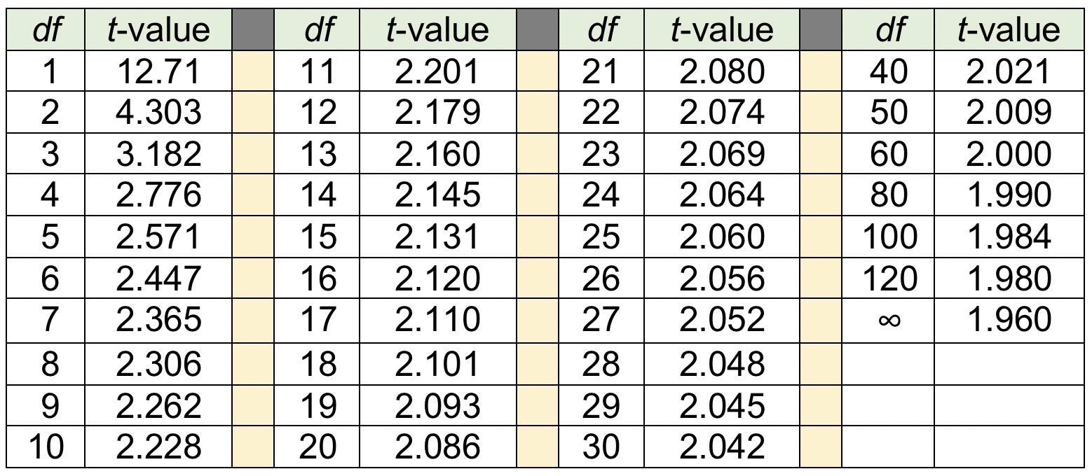
Table of t-distribution. Now we are ready to find the comparison criterion t-value using the standard table mentioned earlier. Table 3-1 present an excerpt of such a table, with only the values for a two-tailed t-distribution at 95% confidence levels. You would read this table by going down the 95% confidence column to the row where the number of degrees of freedom for the sample are presented on the left. The value in that cell would be the t-value against which the computed t-statistic would be compared to draw inferential conclusions.
Table 3-1 presents the values for a two-tailed t-distribution at 95% confidence, depending on the number of observations minus 1 (degrees of freedom). As you can see, the greater the sample size, the greater the number of degrees of freedom, and the greater the number of degrees of freedom, the closer to the population normal distribution value of 1.960 we come. At df=1, we are very far away from that value (12.71 is much greater than 1.960), while at df=30, we are much closer (2.042 is close to 1.960). A full t-table would also include values for other levels of confidence, such as the 90% and 99% levels.
Table 3-1. Values at 95% confidence, for two-tailed t-distribution, by df.

Take a moment to complete the following activity.
Calculating a Confidence Interval for the Mean.
This work has led up to being able to calculate the confidence interval for the population parameter mean from the sample statistic mean. At this point, we simply need to plug the proper values into the appropriate formula and compute the answer. In application, we make two computations using the formula: once to identify the top/highest value in the confidence interval’s range and again to identify the bottom/lowest value in the confidence interval’s range. As a result, we will have identified the range of values based on our sample statistics where, with 95% confidence, the true (unknowable) population mean lies. We will have inferred the population mean from the sample statistics.
Consider what the formula asks us to do. To compute the 95% confidence interval (CI95%) highest value, we start with the sample mean (X̅), then add a computed value that takes into consideration our sample size and the degree of variation observed in the sample values: that computed value is calculated from our t-value (located in the table using our degrees of freedom) multiplied with our standard deviation (sd) which has been divided by the square root of our sample size (√n)–see the formula written below. What that division does is change the overall standard deviation figure into an average degree of variation around the mean—this refers to the formula we used in Chapter 2 to calculate variation and standard deviation in the first place.
Finally, we compute our lowest value in the confidence interval range by doing the same thing but subtracting the computed value instead of adding it. Since we already know the values for everything to the right of X̅ in the formula, we do not have to recalculate it—this time we simply subtract it from X̅ instead of adding.
In mathematical terms, this set of steps looks like this:

Working an Example. This looks a lot more complicated than it really is, so let’s work a simple example. Imagine that the 28 students in our school absenteeism study were drawn randomly from the population of students in a particular school district, and that we safely can assume normal distribution of the days absent across the population of students in an entire school district. From our earlier work, we know the following information:
- X̅=6.93 days absent
- sd=10.452
- n=28
- df=(28-1)=27
- comparison criterion t-value=2.052 (using 27 df at 95% confidence fromTable 3-1)
- square root of 28 = 5.2915 (using a square root computation program)
The highest value in our 95% confidence interval for the population mean would be:
CI95% = 6.93 + [(2.052) * (10.452/√28)]
= 6.93 + [(2.052) * (10.452/5.2915)
= 6.93 + [(2.052) * (1.9752)]
= 6.93 + [4.053]
= 10.98 with rounding.
The lowest value in our 95% confidence interval for the population mean would be:
CI95% = 6.93 – [4.053]
= 2.88 with rounding.
We would report this as: CI95%= (2.88, 10.98). This is interpreted as the school district’s population mean days absent falling between 2.88 and 10.98 days, based on 95% confidence and the sample statistics computed for these 28 students.
Interactive Excel Workbook Activities
Complete the following Workbook Activity:
Chapter Summary
In this chapter, you learned important distinctions between univariate sample statistics and population parameters—that we estimate population parameters using sample statistics. You also learned about strategies for assessing the adequacy of our estimates and our confidence in the how well the sample statistics represent true values for the population. The essential information for developing confidence intervals was presented, including how statisticians select the comparison criterion t-value and degrees of freedom for computing and evaluation results from the statistical formula. A more advanced statistics course could help you better understand the nature of the t-distribution (and how this relates to normal distribution), the rationale behind degrees of freedom, and the assumptions we mentioned in relation to computing confidence intervals. The next chapter examines how some of these concepts apply to bivariate statistical analyses.
